Topics (384k) Articles (398k) Users (410) Discussions (242) Comments (383) Files (13k) New article

A capacitor need not finish discharging before the next pulse arrives. This residual baseline in RC pulse-width discrimination changes the next pulse's RC threshold-crossing time even if its applied height and duration are unchanged. The relaxed-state acceptance formula assumes an initial output of zero; a repeated pulse train can violate that assumption systematically.
Take a first-order RC circuit with time constant , input high level , zero input low level and initial capacitor output . During a pulse of duration ,For , solving for the rising threshold givesA finite interval above threshold requires . At equality the output only touches the threshold at its peak. A positive residual makes the crossing earlier than the zero-baseline crossing. If the output already exceeds the threshold at the start, this rising-crossing formula no longer describes a new edge.
The input of a repeated pulse train is a periodic function with high duration , low duration and period . Put and . The next baseline is the previous peak multiplied by . Writing for the baseline before pulse gives the linear recurrence relationBecause , the deviation from its fixed point is a decaying geometric sequence:This periodic RC pulse-train baseline is a repeatable state of the circuit, rather than random readout noise. In the periodic regime, separate rising and falling comparator transitions require . If , there is no finite high interval. If , there is no finite low interval: missing comparator reset in an RC pulse train can turn repeated input pulses into one sustained output state.
For an original calculation, choose , , , and . An isolated relaxed pulse peaks at only and is rejected. The repeatable train instead hasIts rising threshold occurs after each pulse starts. The falling crossing is , giving an above-threshold duration of . Starting from zero baseline, the first three pulses are rejected, but the fourth peaks at and crosses. A change in pulse acceptance need not mean that the source pulse itself changed.
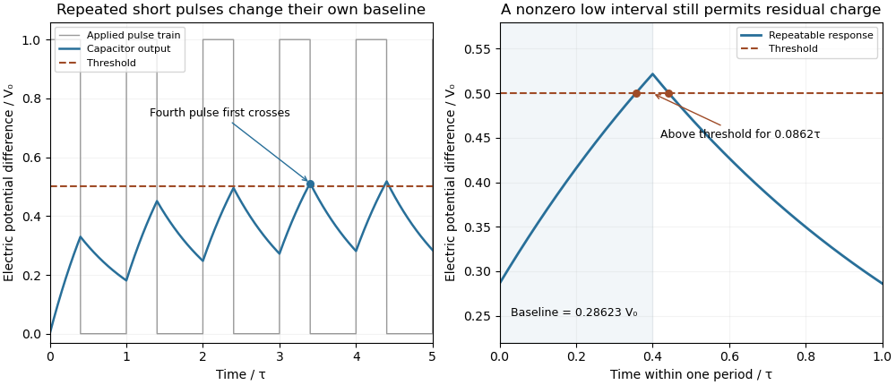
Residual capacitor charge makes a repeated short pulse cross a threshold that rejects the isolated pulse
. Original first-order model, with a 1 µs time constant, 0.4 µs high interval, 0.6 µs low interval and a half-height threshold. The first train starts relaxed; the second panel shows the repeatable baseline and peak. No measured waveforms are used. Details.A useful design bound controls timing error rather than merely calling the circuit discharged. Put and suppose . Relative to the relaxed crossing,Since a nonnegative pulse train in this model has , a low interval guarantees that baseline bound. Combining the inequalities yields a sufficient quiet interval required for an RC baseline timing budget :For a 1% baseline allowance, limits the crossing advance to , or when . The bound is conservative because it uses the largest possible peak.
A bench test holds pulse height, duration and threshold fixed while sweeping repetition period with a pulse generator. Record the actual input and capacitor output on an oscilloscope, including the baseline immediately before each pulse. Probe capacitance and effective source electrical resistance belong in . MIT's laboratory uses repetitive square-wave excitation to measure RC decay, providing a direct way to check the underlying time constant.[ref]
Laboratory 11: Sinusoidal Steady State Response of RC and RL Circuits by MIT OpenCourseWare. Printed pp. 1–2, natural-response and waveform measurements
The calculations above assume ideal input edges and zero input low level; comparator hysteresis and switching dynamics require their own model.Pseudoinverse fitting with a parameter-dependent covariance range requires checking the allowed residual subspace separately for each fitted parameter. If the covariance is and the residual is , the range restriction in singular-covariance spectral fitting becomesThe Moore-Penrose inverse quadratic alone does not enforce this condition. A projector computed at one trial parameter need not describe another trial's allowed noise.
For an original example, let , zero mean and . Noise lies on a line that rotates with . With observation and , the model at permits the observation and gives quadratic value four. At , the pseudoinverse quadratic is zero, yet the observation is outside the allowed vertical line. Minimizing that quadratic without its range constraint would reward an impossible candidate.
The pinned SciPy documentation describes singular-covariance evaluation using pseudo-determinants, pseudoinverses and covariance rank; its implementation additionally applies a numerical support mask and returns zero density, or negative-infinite log density, off support.[ref]
SciPy 1.16.2 documentation. scipy.stats.multivariate_normal, Notes; v1.16.2 scipy/stats/_multivariate.py, _PSD._support_mask and multivariate_normal_gen.pdf/logpdf
Parameter-dependent supports also require care about which measure defines a density. Values defined on different subspaces are not automatically a common likelihood merely because each uses the same-looking formula.A physically justified transverse noise resolves the idealized singularity. With perpendicular unit vector , use . For , the two quadratic values become four and four hundred. The determinant is the same at these orientations, so this full-rank Gaussian model correctly disfavors the transverse observation.
The transverse-noise limit of a rotating rank-one covariance model is an inference about a stated physical noise model, not permission to add arbitrary diagonal noise for numerical convenience. In spectral work, distinguish a parameter-dependent physical noise direction from a fixed deterministic rebinning matrix; the latter has a fixed output range when its input covariance is positive definite.
A rank-one update of pressure-map information describes the extra constraint supplied by one independent scalar pressure measurement. Suppose the existing pressure-map information matrix is , and a new sensor reports with known variance , independent of the existing errors. Adding its squared residual to the weighted least squares objective givesThe added matrix has rank one when . It is positive semidefinite because its quadratic form is . Thus the new observation cannot reduce information in any direction under this fixed linear map and noise model. The noise normalization is the same whitening transformation used to express a correlated residual metric as an ordinary squared norm.[ref]
The update can remove a missing direction only if the new channel actually sees it. More precisely,This follows because a sum of two nonnegative quadratic forms is zero exactly when both are zero. Repeating an existing mixture improves its precision but cannot identify a pressure contrast that all mixtures annihilate.
When is positive definite, write . The Sherman–Morrison formula yields the updated estimator covariance matrixMultiplication by verifies the identity directly. For a particular quantity , its variance falls by . A small noise level is valuable only together with a useful sensitivity direction.
For an original calculation in kilopascal coordinates, let , and . ThenThe variance of the sum drops from to . The negative off-diagonal entry means the two inferred coefficients now have negatively correlated errors; it does not mean either individual variance is negative.
A correlated-channel update of pressure-map information needs the new channel's residual after predicting it from old channel noise. Simply adding double-counts information when a common amplifier or reference contributes correlated errors. A proposed array experiment uses repeated known loads to estimate sensitivity and noise separately, adds one channel, and compares withheld-load errors with . Agreement tests the full assumed model, including independence and unchanged sensor response, rather than the matrix identity alone.
Photoelastic phase unwrapping assigns consistent cycle counts to retardation observations that determine phase only modulo a full cycle. If a phase-resolved method reports , the full relative phase retardation has the formThe integers carry the fringe-order information that the wrapped values omit. A known starting order and sufficiently small changes can make the branch choices recoverable.
For an original one-dimensional example, take wrapped phases radians. Choosing the first value as the known starting branch, the nearby increasing continuation isor approximately radians. The apparent large negative jump is a change of representation at , not a demonstrated physical reversal. The final photoelastic fringe order on this branch is about0.5703.
A nearest-branch rule is justified in a noiseless sequence when successive true phase changes have magnitude strictly below : among increments differing by , exactly one lies in that interval. With phase errors bounded by , the stronger condition is sufficient for that local choice. Larger steps, discontinuities or inadequate signal can cause a photoelastic branch-slip error. One wrong cycle changes inferred stress-difference magnitude by in the uniform-specimen model.
The algorithm assumes phase or equivalent branch information is available. A single crossed-polarizer intensity does not itself supply a unique signed wrapped phase. Its ambiguity includes reflection within a cycle as well as the integer count. Additional polarization measurements, a known load path or other reference information must justify phase recovery before applying the simple continuation rule. The primary stress-analysis derivation explicitly shows how intensity depends on retardation and axis orientation.[ref]
Experimental Strain Analysis by David Roylance. Printed pp.6–8, analyzer transmission and fringe interpretation
The Illinois apparatus supplies controlled loading, a load-cell record and camera observations, making a load-indexed sequence physically meaningful.[ref]
Polariscope and Photoelasticity by the University of Illinois Mechanical Testing Instructional Laboratory. Manual leadscrew/load readout and camera observation
Continuity alone still leaves a common offset unless the absolute starting order is known. An unloaded image can reveal residual retardation rather than automatically establish zero stress or zero order.A multi-sample clearance envelope bounds every possible instantaneous clearance consistent with several uncertain distance queries and a known motion-rate limit. It sharpens isolated endpoint estimates by requiring one Lipschitz continuous clearance history to explain all samples. Such a bound addresses the between-sample gap in continuous robot motion planning, where valid sampled configurations alone do not guarantee a valid path.[ref]
Robotic Systems by Kris Hauser. Chapter 8, Point-to-point path planning; Chapter 9, configuration-space obstacles
At times , let , and suppose the nonnegative clearance has Lipschitz constant . Assuming multi-sample consistency of distance-query intervals, defineEvery admissible history obeys . Each lower cone follows from ; the upper cones follow by reversing the inequality. Under consistency, both envelope functions themselves satisfy the sample intervals and the same Lipschitz bound. Thus the enclosure is pointwise sharp among the scalar histories allowed by these assumptions.
A positive minimum of over a time interval certifies separation throughout it. If that minimum is zero, the assumptions permit a scalar history touching zero; this is lack of a strictly positive certificate, not an observation of collision. Some admissible scalar histories may not correspond to a realizable rigid-body path, so sharpness here concerns the stated scalar model.
The exact interval minimum is inexpensive to compute. On , all sample times lie on one side or the other. PutThen . For , its minimum occurs at the crossing if that crossing lies in the interval; otherwise it occurs at the nearer endpoint. Prefix and suffix maxima therefore allow all segment minima to be computed in linear time. For , every admissible clearance is constant and the lower envelope is .
For an original example, queries at give intervals , , , and . On the first segment, and in the corresponding millimetre/second coordinates. The crossing is and the lower bound there is . Symmetry gives a second minimum at , so the full interval is certified with margin . Using only the two outer queries would give a minimum of .
A proposed checker first tests consistency, then computes segment minima with conservative arithmetic and reports the limiting time and active queries. Keep query errors, timestamps and the bound traceable to the same geometry and motion. Clearance envelope with segment-dependent speed bounds can use more motion information, but replacing by an unsupported smaller number would invalidate the certificate.
The noise cost of polynomial baseline cancellation is the change in random measurement uncertainty when extra background trends are removed. For a linear pulse estimate and reading-error covariance matrix ,The moment conditions for baseline-drift cancellation constrain to reject specified polynomial backgrounds. They do not make the remaining random error vanish.[ref]
For an original comparison, assume a pulse occupies only the central sample and the other samples contain background alone. Three samples at with weights cancel constant and linear backgrounds. Five samples at can instead useThese weights preserve the central signal and have zero moments of orders . For independent reading errors of equal variance , the three-sample variance is , while the five-sample variance isWith and , the standard uncertainties are approximately and . The second design removes quadratic and cubic drift as well, but its larger reference weights increase noise. This compares two specified estimators; it is not a claim that collecting more background data must worsen precision.
NIST's pulse-energy apparatus used before/after baseline measurements for background and thermal-drift correction.[ref]
Calibration Service for Low-level Pulsed-Laser Radiometers at 1.06 µm: Pulse Energy and Peak Power by Rodney W. Leonhardt. §3.5, printed p. 8; §7.2, Leakage Effect
The polynomial comparison above is an original model for choosing such measurements. Choosing minimum-noise weights under baseline moment constraints can exploit additional reference samples and their measured correlations. Pulse leakage into a reference or drift outside the cancelled polynomial family still creates bias.The noise penalty from nearly parallel signal and reference shapes is the precision lost when a spectral estimator must reject a nuisance pattern resembling its desired signal. For nonzero shapes and positive-definite noise covariance , define their inverse-covariance correlationThe Cauchy-Schwarz inequality gives . The minimum-variance spectral contrast orthogonal to a reference shape has varianceIf the nuisance amplitude were known and subtracted without uncertainty, the corresponding optimum variance would be . Exact nuisance rejection therefore multiplies variance by and standard uncertainty by .
The relevant angle is the noise-whitened angle between spectral signal and nuisance shapes: it is measured after a whitening transformation, not generally from the raw plotted spectra. A channel with large noise contributes little to separating the shapes even if their plotted curves differ there.
For an original example, let , and . Rejecting the reference forces the contrast to , with variance . With known nuisance amplitude, its variance would be . The rejection penalty is therefore in variance, about in standard uncertainty. Only the weak second-channel component distinguishes signal from nuisance.
The primary stimulated-Raman experiment reported systematic spectral noise above its calculated shot-noise limit and described pure-solvent subtraction of a common pattern.[ref]
Femtosecond Broadband Stimulated Raman: A New Approach for High-Performance Vibrational Spectroscopy by David W. McCamant and others. Results and Discussion, theoretical shot-noise limit versus observed noise and pure-solvent subtraction
A reference can remove that shared pattern while also making an overlapping desired signal hard to estimate. Retain full covariance in the variance calculation.[ref]Guidelines for Evaluating and Expressing the Uncertainty of NIST Measurement Results by Barry N. Taylor and Chris E. Kuyatt. Appendix A, equation A-3
At exact proportionality, no unit-response rejecting contrast exists; a low-noise result obtained by suppressing the signal as well is not a valid amplitude estimate.Deer are mammals of the family Cervidae. They include species with bony antlers that are shed and regrown, and their browsing can strongly influence vegetation. Family membership, external appearance and the ancestry of an individual are related but different kinds of information.
A genetic study of red and introduced sika deer in Scotland combined microsatellite markers with mitochondrial DNA. Two broadly distinct genetic groups persisted, yet introgressed alleles were detected where their distributions overlapped. [ref]
Introgression through rare hybridization: A genetic study of a hybrid zone between red and sika deer (genus Cervus) in Argyll, Scotland by Simon J. Goodman and others. 1999, abstract: eleven microsatellite markers, mitochondrial DNA and introgression
Thus recognizable groups can exchange some genes without becoming immediately indistinguishable. Appearance alone need not reveal every episode of ancestry across a hybrid zone.An ungulate is conventionally a hoofed mammal. The name has also been applied broadly to extinct mammals with superficially similar anatomy, so a historical grouping by body form need not specify one exact modern evolutionary lineage. Convergent traits can make fossil relationships difficult to infer.
Ancient-protein analysis tested the relationships of two enigmatic South American forms. Collagen sequences recovered from fossils were compared with sequences from living mammals, placing the sampled extinct taxa near the odd-toed ungulate lineage rather than the alternative placements suggested by some anatomical comparisons. [ref]
Ancient proteins resolve the evolutionary history of Darwin's South American ungulates by Frido Welker and others. 2015, abstract: fossil collagen sequence recovery and phylogenetic placement of Toxodon and Macrauchenia
Molecular preservation thereby supplied evidence complementary to shape, even where recoverable ancient DNA had been lacking.Peromyscus is a genus of primarily New World rodents, including animals commonly called deer mice. It is distinct from the genus of the house mouse and has become useful for studying variation in ecology, behaviour and reproduction among related species.
Crosses between two Peromyscus species produced growth differences depending on which species supplied the mother and father. Analysis found disruption of genomic imprinting in the hybrids, while imprinting remained present in the tested parental species. [ref]
Genomic imprinting is disrupted in interspecific Peromyscus hybrids by Paul B. Vrana and others. 1998, abstract: reciprocal species crosses, growth effects and disrupted hybrid imprinting
The result distinguishes a hybrid regulatory mismatch from complete absence of the mechanism in one parent. Swapping the direction of a cross can expose parent-of-origin effects hidden by a single pooled hybrid category.The cat, Felis catus, is a domesticated mammal in Carnivora. The name here refers to the domestic species, rather than every wild member of the broader cat family. Coat patterns and named breeds vary within the domestic species; a breed is not automatically a separate species.[ref]
Cats provide a useful example of how ancestry is investigated with DNA. A 2007 study compared 979 domestic and wild cats using mitochondria-associated DNA and nuclear genetic markers, including microsatellites. Domestic samples clustered with the sampled Near Eastern wildcat lineage, supporting ancestry from that population rather than an origin independently from every regional wildcat population.[ref]
The Near Eastern origin of cat domestication by Carlos A. Driscoll and others. Abstract; sampling and genetic-clustering analyses
This is a comparison of inherited variation, not a direct measurement of the moment a wild animal became a domestic one. A phylogenetic tree can connect sampled populations while the cultural process of domestication extends across many generations. Similarly, a cat living away from people is not thereby a different species: present living conditions and genetic ancestry answer different questions.
A wildcat in the narrower zoological usage is one of the closely related wild Felis lineages resembling the domestic cat. Current Cat Specialist Group taxonomy distinguishes the European wildcat, Felis silvestris, from the Afro-Asiatic wildcat, Felis lybica, and from the domestic cat, Felis catus. Older literature sometimes grouped several of these lineages within a broadly defined Felis silvestris. A feral cat is a free-living domestic cat, so living without human care does not alone identify an animal as a wildcat.[ref]
European wildcat species account by the IUCN SSC Cat Specialist Group. Taxonomy section: recognized Felis species
Genetic markers can investigate ancestry beyond outward resemblance. A 2007 study by Carlos A. Driscoll and collaborators assessed 979 domestic and wild cats, comparing microsatellites and DNA sequences from mitochondria. The sampled domestic lineages clustered closely with Near Eastern wildcats. The paper's own subspecies names should be read in its historical classification, rather than silently replaced with a modern species list.[ref]
The Near Eastern origin of cat domestication by Carlos A. Driscoll and others. Abstract; Figures1–2: sampling, nuclear markers and mitochondrial lineages
The comparison separates two questions: what ancestry the sampled animals share, and what taxonomic rank to assign each lineage. Hybridization with domestic cats can further complicate identification, making one coat pattern or one inherited marker an incomplete description of an individual animal.
Felis is a taxonomic genus within Felidae, the cat family in Carnivora. It includes the domestic cat and several small wild species, including the European wildcat and Afro-Asiatic wildcat. Thus Felis is broader than the domestic species Felis catus but narrower than the entire family of cats.[ref]
This hierarchy makes an identification example useful. A specimen identified only as Felis has been assigned to a taxonomic genus, not necessarily identified as a domestic cat. Conversely, a cat does not leave Felis when it begins living independently of people. Taxonomic membership and current living conditions answer different questions.
The distinction also matters when comparing DNA. Regional wildcat lineages can share close ancestry and undergo hybridization without every comparison using the same species boundaries. A study's names should be interpreted with its stated classification and sampling, especially when older accounts placed several lineages within one broad wildcat species.
The guinea pig is the domestic rodent species Cavia porcellus. NCBI Taxonomy places it in the genus Cavia and family Caviidae within Rodentia. Its common name does not place it among pigs. A species name identifies the organism used in a study; it does not specify the strain, tissue preparation or physiological measurement.[ref]
Cavia porcellus in NCBI Taxonomy. TaxID10141, scientific/common names and lineage
A motivating experimental example comes from a1968 complement C5 study. Investigators separated an active fragment from guinea-pig material and tested biological responses, including activity in guinea-pig ileum and chemotaxis of rabbit leukocytes. Keeping the source species, assay species and measured response explicit prevents treating these as one interchangeable readout.[ref]
Chemotactic and anaphylatoxic fragment cleaved from the fifth component of guinea pig complement by H. S. Shin and others. Abstract; separated C5 fragment and tissue/cell assays
For an invented tissue-response comparison, a preparation contracts by2 millimetres before treatment and5 millimetres afterward. The difference is3 millimetres, and the second displacement is2.5times the first. Those calculations describe that preparation and instrument setting. They do not establish an equivalent whole-animal response, a human dose or the molecular identity of every active component. The organism, preparation and endpoint are all parts of the experiment.
Lacertidae is a family of lizards within Lacertoidea, distinct from Teiidae, Gymnophthalmidae and amphisbaenians. It provides an important comparison for the latter group: common ancestry can connect normally limbed lizards with highly modified burrowing forms, so a wormlike body is not by itself a reliable map of evolutionary relationships.[ref]
Lacertidae is also a useful system for investigating thermoregulation. A 2019 comparative study related environmental temperatures to thermal physiology and to the evolutionary histories inferred from genomic data. Behavioral choices, such as basking or using shaded shelter, are relevant because the air temperature at a site is not automatically an animal's body temperature.[ref]
Environmental temperatures shape thermal physiology as well as diversification and genome-wide substitution rates in lizards by Joan Garcia-Porta and others. thermal physiology, preferred temperatures and discussion of basking
For an illustrative measurement design, offer a lizard a range of warm and cool positions and record both its chosen position and body temperature. Repeating the assay at different background temperatures distinguishes an available environment from the temperature the animal actively selects. Comparisons between species then require the same measurement protocol and an account of their relatedness; otherwise a difference caused by the assay or shared ancestry can be mistaken for an independent adaptation.
Teiidae is a family of lizards within Lacertoidea, including the whiptails of Aspidoscelis. It is a separate lineage from Gymnophthalmidae. Beyond their place in reptile classification, some whiptails offer a striking example of parthenogenesis: females produce offspring without fertilization.[ref]
In a 2010 study of parthenogenetic Aspidoscelis, investigators asked how eggs could retain the parental complement of chromosomes and preserve heterozygosity. Chromosome imaging and fluorescent probes showed an extra premeiotic doubling, followed by pairing of genetically identical chromosome copies. The cells still underwent meiosis and chromosomal crossover; reproduction did not simply bypass the entire meiotic program.[ref]
A simplified genetic example explains the significance. Begin with distinguishable chromosome versions and . After copying, matching with another and with another permits exchange between equivalent copies while retaining both parental versions in the unreduced egg. This differs from mechanisms that discard one version and thereby lose heterozygosity. The finding concerns particular parthenogenetic species; it does not make every member of Teiidae an asexual animal.
Gymnophthalmidae is a family of lizards within Lacertoidea, often called microteiids. It is distinct from Teiidae, despite that historical common name. Its members include forms with fairly conventional limbs and forms with strongly reduced limbs and elongated bodies, making the family useful for studying how a body plan changes during evolution.[ref]
A morphological study distinguished modest reductions, such as losing one or two finger or toe bones, from much more extensive reductions that can leave no externally distinct adult limb. The investigators compared digit arrangements and also examined gene expression in developing reduced limbs. Adult anatomy and embryonic development consequently provide complementary observations of the same evolutionary problem.[ref]
Digit evolution in gymnophthalmid lizards by Juliana G. Roscito and others. abstract, two groups of reduced limb morphologies and embryonic gene expression
For an anatomical example, two feet can each have four visible digits while differing in which digit is absent or in the number of bones within each remaining digit. Merely counting visible toes collapses those possibilities into one score. Recording the detailed bone pattern and placing it on a phylogenetic tree gives a more informative test of whether superficially similar reductions share an evolutionary origin.
Finite-input correction in pulse-detector calibration removes the known input duration from an inferred receiver width, while propagating uncertainty in both widths. Under the nonnegative, normalized, finite-variance convolution model of known-input calibration of a pulse detector,where is the known input profile, the measured output and the receiver's impulse response. The subtraction concerns temporal variances, not arbitrary reported full widths.
Differentiating on the positive-width branch givesFirst-order propagation of standard uncertainty therefore yieldsThe covariance matters when both widths use the same timebase or fitted reference.[ref]
An original near-resolution example has and , each with independent standard uncertainty . The corrected receiver width is and its propagated standard uncertainty is about , or . Width measurements individually precise to about one percent can thus give a much less precise difference-derived width.
NIST's primary bandwidth-correction procedure used roughly 120 ps optical inputs and recorded the detector, cable and oscilloscope as one response chain at different gains and signal levels.[ref]
Calibration Service for Low-level Pulsed-Laser Radiometers at 1.06 µm: Pulse Energy and Peak Power by Rodney W. Leonhardt. Appendix C.1–C.2, printed pp. 36–37, Figure C1 and steps 1–7
A sufficiently short characterized input reduces this resolution-limit conditioning in finite-input detector calibration. Near a zero variance difference, linear uncertainty propagation may fail; a nonpositive measured difference does not represent a negative physical detector width. Report an interval or limit under the stated model rather than silently replacing the difference by zero. Negative ringing also violates the nonnegative-profile assumption behind the variance subtraction.Boundary-sensitive Gaussian overlap inversion describes the loss of stable radius information when a symmetric log-overlap ratio approaches its finite-model limit. A central reading can remain formally invertible while small measurement uncertainty reaches values for which no finite radius ratio exists.
For known , define , andThe inversion of a symmetric Gaussian overlap log-ratio requires . At the upper limit , the radius ratio tends to zero; at the lower limit it tends to infinity.
An original expansion near the upper limit puts . Expanding the hyperbolic tangent givesThus the approximate relative radius uncertainty is when linearization is still justified. The distance to the boundary, rather than the magnitude of alone, controls this sensitivity.
For stipulated and a central log-ratio only 0.01 below , the asymptotic radius ratio is about 0.0365. A standard uncertainty 0.02 in is twice the boundary distance, so a small symmetric error bar on the inferred radius is not credible. In a hypothetical Gaussian readout model centered there, roughly 31% of readings fall beyond the finite-inversion limit. This is a statistical illustration, not an observed receiver distribution.
Interval propagation for bounded overlap data shows the asymmetry directly. A stated interval in that reaches the upper bound maps to radius ratios arbitrarily close to zero; it does not yield a symmetric finite relative interval. An interval wholly inside the domain maps monotonically, with its endpoint order reversed.
Discarding out-of-range Monte Carlo draws would condition on a selected subset and change the distribution being propagated. Instead, examine the forward measurement model, admissible parameter range and calibration uncertainty, or construct an explicitly stated inference using the measured data. JCGM 101 separates input-distribution assignment from numerical propagation and states conditions for valid Monte Carlo use.[ref]
Finally, proximity to the mathematical boundary is not the only possible problem. A change in shared normalization, polarization or wavefront curvature can violate the one-radius model. NIST's receiver apparatus illustrates the need for optical matching and separate electrical corrections.[ref] Numerical clipping cannot replace those physical checks.
A current-plane convention in heterodyne calibration specifies which electrical current an inferred beat amplitude denotes: the detector's generated small-signal current, the current entering a cable, or the current dissipating power in a particular load. Those amplitudes need not be equal. A power-to-current conversion is meaningful only with its circuit and reference plane.
An original photodiode model uses generated peak-current phasor , detector shunt admittance and load impedance . Kirchhoff's current balance givesThe factor one half assumes peak phasors; with RMS phasors it disappears. The current in the load determines delivered electric power. The generated current is recovered only after correcting the current division and any intervening network.
For a resistive Norton model with source resistance and load resistance both , , so and . If the source shunt admittance is negligible, instead. Calling both circuits “a detector feeding a 50-ohm instrument” does not establish the same current conversion.
Capacitive current division in heterodyne receivers adds frequency dependence. With and resistive load ,For stipulated pF and , this magnitude is approximately 0.9540 at 1 GHz and 0.3033 at 10 GHz. The same generated amplitude then gives a smaller measured load current at the higher frequency. These are equivalent-circuit calculations, not measured specifications of a particular photodiode.
NIST's primary optical-receiver experiment distinguishes microwave power delivered to a reference load from the power indicated by a sensor. It corrects sensor calibration, interconnecting-network loss and impedance mismatch using measured scattering and reflection parameters.[ref]
Frequency response metrology for high-speed optical receivers by Paul D. Hale and others. PDF pp. 1–2, Eqs. 1–4 and Fig. 1
That apparatus makes the reference plane an experimental calibration choice rather than a label applied after analysis.Document the detector model, load, frequency, cable and connector corrections, and peak-versus-root mean square convention before normalizing by separate arm currents. If the arm currents describe generated DC photocurrent while the beat numerator describes uncorrected load current, the resulting overlap includes electrical current division. Heterodyne amplitude-versus-power gain conversion and impedance matching address different parts of that chain and both may be needed.
Pinned article: Introduction to the OurBigBook Project
Welcome to the OurBigBook Project! Our goal is to create the perfect publishing platform for STEM subjects, and get university-level students to write the best free STEM tutorials ever.
Everyone is welcome to create an account and play with the site: ourbigbook.com/go/register. We belive that students themselves can write amazing tutorials, but teachers are welcome too. You can write about anything you want, it doesn't have to be STEM or even educational. Silly test content is very welcome and you won't be penalized in any way. Just keep it legal!
Intro to OurBigBook
. Source. We have two killer features:
- topics: topics group articles by different users with the same title, e.g. here is the topic for the "Fundamental Theorem of Calculus" ourbigbook.com/go/topic/fundamental-theorem-of-calculusArticles of different users are sorted by upvote within each article page. This feature is a bit like:
- a Wikipedia where each user can have their own version of each article
- a Q&A website like Stack Overflow, where multiple people can give their views on a given topic, and the best ones are sorted by upvote. Except you don't need to wait for someone to ask first, and any topic goes, no matter how narrow or broad
This feature makes it possible for readers to find better explanations of any topic created by other writers. And it allows writers to create an explanation in a place that readers might actually find it.
Figure 1. Screenshot of the "Derivative" topic page. View it live at: ourbigbook.com/go/topic/derivativeVideo 2. OurBigBook Web topics demo. Source. - local editing: you can store all your personal knowledge base content locally in a plaintext markup format that can be edited locally and published either:This way you can be sure that even if OurBigBook.com were to go down one day (which we have no plans to do as it is quite cheap to host!), your content will still be perfectly readable as a static site.
- to OurBigBook.com to get awesome multi-user features like topics and likes
- as HTML files to a static website, which you can host yourself for free on many external providers like GitHub Pages, and remain in full control

Figure 2. You can publish local OurBigBook lightweight markup files to either OurBigBook.com or as a static website.
Figure 3. Visual Studio Code extension installation.
Figure 5. . You can also edit articles on the Web editor without installing anything locally. Video 3. Edit locally and publish demo. Source. This shows editing OurBigBook Markup and publishing it using the Visual Studio Code extension. 
- Infinitely deep tables of contents:



All our software is open source and hosted at: github.com/ourbigbook/ourbigbook
Further documentation can be found at: docs.ourbigbook.com
Feel free to reach our to us for any help or suggestions: docs.ourbigbook.com/#contact