Topics (384k) Articles (398k) Users (410) Discussions (242) Comments (383) Files (13k) New article

Tie-line phase-fraction sensitivity measures how an inferred phase fraction changes when the overall composition or the measured liquid-liquid tie line endpoints change. A sensitivity coefficient is a local partial derivative of the inference formula, rather than an uncertainty by itself. It becomes an uncertainty contribution only after combination with the input covariance matrix.[ref]
Guide to the expression of uncertainty in measurement by JCGM. §§5.1.3–5.1.4, sensitivity coefficients and their experimental determination
For one composition coordinate of a binary mixture, write the lever rule aswhere are endpoint mole fractions, is the overall mole fraction and is the mole-based amount of phase . Differentiating the mass balance givesThus a measurement error in the overall composition and an equal measurement error in the phase- endpoint have different effects. The conditioning of tie-line phase-fraction inference deteriorates as the endpoint separation becomes small: the same composition measurement error then produces a larger change in the inferred phase fraction.
For an original example, take , , , giving . Increasing only by gives a first-order change . Direct substitution gives , a change of . For the closer endpoints , and balanced composition , the local sensitivity to the same endpoint error is ten times larger. This is a property of the inference geometry; it does not establish whether either hypothetical pair is in liquid-liquid equilibrium.
The multidimensional tie-line phase-fraction fit has an additional detail away from an exactly balanced composition. On independent mole fraction coordinates, hold a symmetric positive-definite matrix fixed and definewith distinct endpoints. Define row vectors and . Differentiating the generalized least squares normal equation givesThe residual correction in tie-line sensitivity vanishes when . Otherwise, moving an endpoint also rotates the fitted line relative to the nonzero ternary tie-line consistency residual. Omitting that contribution is an additional approximation. If itself changes with the measured inputs, its derivative must also enter the calculation.
These formulas describe the unconstrained fit locally. Imposing introduces boundary effects, and coincident endpoints make this inference undefined. A practical sensitivity check recomputes the fit after small positive and negative perturbations of one measured coordinate, keeping composition closure and the stated weight matrix. Agreement as the perturbation shrinks tests the derivative calculation; it does not validate the underlying equilibrium model.
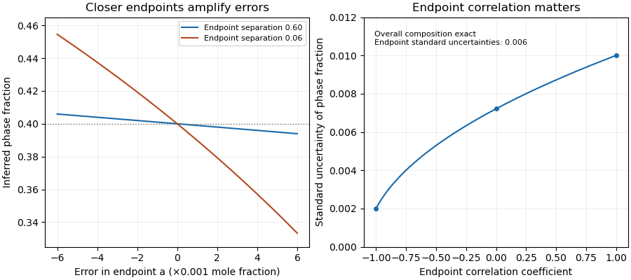
Closer tie-line endpoints amplify composition errors; endpoint correlation changes the inferred phase-fraction uncertainty
. Original binary examples with phase fraction0.40. Left: exact endpoint perturbations at separations0.60 and0.06. Right: first-order standard uncertainty with uncertain endpoints and exact overall composition; common calibration of all three measurements is a different model. Details.A shot-resolved pulse-contrast estimator normalizes each individual optical shot before combining its contrast with other shots. For a specified side-delay signal and positive central signal , both background-corrected, defineThe estimand is the mean of the individual shot ratios under the stated sampling and acceptance rule. It differs from normalizing an accumulated trace, , which has third-order correlation brightness weighting.
An original three-shot example uses central signals and side signals . The individual ratios are , with equal-shot mean about 0.0433. Normalizing the sums gives . The latter gives the brightest shot most of the influence. Both are valid summaries of the chosen data, but answer different questions.
Single-shot acquisition matters when the profile fluctuates. The primary third-order correlator maps delay into a spatially resolved signal and records it on a CCD, using second-harmonic generation and sum-frequency generation to form the gate.[ref]
A Single Shot 3rd Order Cross-Correlator for Pulse Contrast and Pulse Shape Measurements by J. Collier and others. printed pp. 194–195, Description and Fig. 2
A scanned trace assembled from different shots does not by itself provide all the for a common ensemble.Normalization introduces pulse-contrast ratio denominator noise. First-order uncertainty propagation for one ratio givesShared baseline estimates can correlate the numerator and denominator, so their covariance cannot automatically be set to zero.[ref]
Guide to the expression of uncertainty in measurement by JCGM. §§5.1–5.2, sensitivity coefficients and correlated inputs
For stipulated , , independent and , the local approximation gives and . Near a zero or poorly resolved denominator the linear approximation and even a finite mean ratio may fail. A central-signal acceptance threshold changes the selected ensemble and must be reported.
For independent shots with a well-behaved ratio distribution, sampling uncertainty in the equal-shot mean can be estimated from the observed ratio variation. Consecutive shots may instead share drift, calibration errors or correlated pulse fluctuations. Keep the acquisition timing, background treatment, saturation checks and rejected-shot count with the estimate; averaging cannot repair an undefined denominator or an unspecified selection rule.
Aspidoscelis is a taxonomic genus of whiptail lizards in Teiidae. It contains both sexually reproducing species and all-female lineages that reproduce by parthenogenesis. This variation makes a closely related set of animals useful for studying how reproduction and chromosome organization interact.[ref]
Sister chromosome pairing maintains heterozygosity in parthenogenetic lizards by Aracely A. Lutes and others. Abstract, sexual and parthenogenetic whiptails
In a 2011 experiment, researchers crossed a triploid parthenogenetic female lineage with males of a sexually reproducing lineage. The resulting four-copy hybrid offspring were checked with molecular and chromosome measurements. Some female offspring themselves reproduced by parthenogenesis, establishing laboratory lineages able to reproduce without repeating the original cross.[ref]
Laboratory synthesis of an independently reproducing vertebrate species by Aracely A. Lutes and others. Abstract and Results, tetraploid hybrids and independent reproduction
A chromosome-set calculation clarifies the change: an unreduced egg carrying three sets can combine with a sperm carrying one set to make a four-set offspring, . This is tetraploidy, rather than merely four copies of one selected gene. Producing one viable hybrid is also different from demonstrating that its descendants can reproduce. The experiment tested both steps, linking the immediate effects of a cross to the persistence of a new reproductive lineage.
Rare-thickness leverage on inverse moments is the disproportionate contribution of uncommon, very thin layers to inferred density when . Its sampling consequence is especially revealing: a sample can miss the influential component and report very little apparent variability.
Consider an original two-point thickness model. Let the rare thickness be with probability , and the common thickness be otherwise. Define and . Among independent measurements the rare count has a binomial distribution, and the estimated mean reciprocal thickness isConsequently,Multiplication by converts these into the mean and variance of the sample mean inferred density. The formulas are exact for this constructed model.
Take , micrometres and micrometres. The true mean reciprocal thickness is approximately . With , zero rare observations has probability about 0.905 and gives . Exactly one rare observation instead gives . The sampling distribution is highly asymmetric despite the large-looking sample count. When every sampled value is the same common thickness, the ordinary sample variance is even zero; it has not revealed the missing component.
Rare-event discovery versus inverse-moment precision distinguishes two experimental objectives. To have at least 95% probability of seeing one rare event requiresor 29,956 observations for this . Estimating the rare fraction to relative standard uncertainty about 10% instead needs roughly one million independent observations, since . Seeing one event is not precise quantification of its contribution.
A distributional assumption therefore needs physical support near zero thickness, not just a fit to the sample centre. NIST's gamma distribution and lognormal distribution entries specify distinct lower-tail models; choosing either is a modeling decision.[ref] Dimensional resolution and independent geometric bounds can be more informative than extending a simulation that never challenges its assumed tail.
Reference-state transfer in overlap normalization uses a known optical state to estimate a state-dependent instrumental offset, then transfers that correction to the specimen measurement. Its central assumption is that the relevant state-gain ratio remains applicable between the reference and specimen. Repeatability of the reference alone does not establish transfer.
Let , andSuppose specimen and reference observations satisfyWith known reference state , the corrected specimen log-ratio isThe residual is exactly the failure of the instrumental offset to transfer. Acquisition order can address time drift, but cannot by itself prove .
An original matched-state example has and . If the specimen's state-gain ratio differs from the reference's by , the corrected ratio still contains 0.02. Ignoring that residual gives an inferred radius ratio approximately 0.9917 instead of one. Repeating both measurements can reduce independent scatter while preserving that systematic offset.
Reference uncertainty must also propagate. Near a matched reference, . For , its magnitude is 2.4. A standard uncertainty 0.01 in the reference log-radius therefore contributes 0.024 to the corrected log-ratio before combining other errors. If the same reference estimate corrects many specimens, this uncertainty is shared; it does not become independent for each specimen. The GUM explicitly retains covariance from common references.[ref]
Operating-point transfer of an overlap reference requires checking the variables capable of changing the state response: optical power, detector bias, electronic range, frequency and illumination. A useful proposed test brackets specimen readings with reference readings and repeats the reference at several operating powers. A trend then tests a transfer assumption; an unchanged reference at only one power leaves power-dependent transfer untested.
NIST's receiver apparatus controls spatial mode and polarization with a polarizer and single-mode-fibre coupling, while separately calibrating the electrical response.[ref]
Frequency response metrology for high-speed optical receivers by Paul D. Hale and others. PDF p. 1, Heterodyne measurements
A reference must preserve the relevant optical and electrical conditions, or the analysis must model their differences. The transfer calculation above is an original diagnostic construction, not a claimed NIST protocol.A periodic RC pulse-train baseline is the repeatable pre-pulse capacitor voltage reached after startup. It need not be zero even when the input low level is zero. With high duration , low duration , period , and , , the recurrence in residual baseline in RC pulse-width discrimination has contraction factor . Its fixed baseline and peak areThis is a deterministic periodic state, not a random noise floor. The startup error is reduced by a specified fraction after cycles, rounded upward.
The mean supplies an independent check. Integrating over a full period makes the derivative term vanish, so . The mean depends on duty cycle while the baseline and ripple depend on period relative to the time constant. For at fixed , expansion givesThus a rapid train approaches a level near its duty-cycle average, rather than isolated relaxed pulses.
For an original fast-train example, choose , , and . The exact baseline is about , the peak , and the mean exactly . The startup deviation contracts by each cycle; reducing it below one percent of its initial value takes 24 cycles, or .
A pulse-generator/oscilloscope test should therefore distinguish the first pulses from the repeatable train, and record minima, maxima and mean rather than only input width. The natural-response measurement in the primary RC laboratory checks the time constant used here.[ref]
Laboratory 11: Sinusoidal Steady State Response of RC and RL Circuits by MIT OpenCourseWare. Printed pp. 1–2
Threshold placement relative to the repeatable minimum and maximum determines acceptance and missing comparator reset in an RC pulse train.Missing comparator reset in an RC pulse train occurs when the filtered output never spends a finite interval below the reset threshold between pulses. In the periodic first-order model, with and , the baseline is the minimum output and equalsFor a nonhysteretic ideal electronic comparator with , leaves no finite low interval. At equality the waveform merely touches the threshold. This is different from a pulse whose peak never reaches threshold and therefore gives no finite high interval.
Solving the strict reset condition givesSeparate rising and falling transitions also require the peak to exceed the threshold. Both inequalities matter, so increasing the quiet interval is not automatically sufficient to produce an accepted output pulse from a weak input.
For an original three-regime example, take , , and . The reset boundary is . At , the periodic baseline/peak are about : after startup the electronic comparator does not reset. At , they are , allowing both transitions. At , the peak is only about , so no finite high interval is produced. The same input height and high duration can therefore give three different output patterns as repetition changes.
The threshold-reset margin for a periodic RC pulse train must also accommodate uncertainty and switching dynamics. With a Schmitt trigger, the lower switching threshold controls reset while the upper one controls acceptance. The capacitor-level inequalities alone do not specify propagation delay or a real electronic comparator's minimum switching dwell time.
A test records the source, capacitor output and electronic comparator output together while sweeping . A steady high output with a pulsing input should be compared with the measured capacitor minimum before being attributed to a source failure. The RC decay model can be checked independently using the primary laboratory's natural-response method.[ref]
The quiet interval required for an RC baseline timing budget controls how much a residual capacitor baseline may advance the next threshold crossing. In residual baseline in RC pulse-width discrimination, a positive baseline changes the relaxed crossing byFor a permitted advance , requiring is equivalent to , where . To retain a fresh rising crossing, also require , equivalently .
After a previous peak , a zero-input low interval gives . Hence a measured upper bound on that peak gives the sufficient intervalUsing only the model bound recovers the conservative expression in the header, . The peak bound and initial-state assumptions are part of the guarantee. The next pulse must still last long enough to produce the rising crossing; this timing bound alone does not guarantee acceptance.
For an original timing budget, let , and . Then , and the conservative interval is . If a validated peak bound is only , it reduces to . Simply calling either interval several time constants long would hide the actual timing specification.
For , expansion gives under the full-height peak bound. Tightening a small timing allowance by a factor of two therefore adds roughly of quiet time. If the allowed advance is as large as the whole relaxed crossing time, a separate reset condition is still required; the logarithmic timing budget alone no longer ensures the initial output is below threshold.
A bench test measures the peak and the baseline while sweeping the low interval, keeping the threshold and pulse height fixed. MIT's RC laboratory supplies the natural-decay measurement used to check the underlying time constant.[ref]
Laboratory 11: Sinusoidal Steady State Response of RC and RL Circuits by MIT OpenCourseWare. Printed pp. 1–2, repetitive excitation and RC decay
Probe capacitance and source resistance belong in that measured time constant.The transverse-noise limit of a rotating rank-one covariance model describes how an ordinary two-dimensional noise distribution concentrates onto a line as one physical noise scale tends to zero. For orthonormal vectors , setA zero-mean Gaussian observation has densityThe pseudoinverse fitting with a parameter-dependent covariance range article explains the range restriction at the exactly singular endpoint.
For a fixed point off the line, , the exponential drives this density to zero as . On the line the two-dimensional density grows like . There is no finite pointwise two-dimensional density limit: probability concentrates onto a one-dimensional Gaussian measure. A density on that line uses a different reference measure. Simply substituting zero for in the full-rank density formula is invalid.
For an original angular example, let an observed vector have length along orientation , with and . At angular displacement ,At radians the density ratio is about . The angular resolution set by transverse spectral noise has characteristic small-angle scale radians, or , when the transverse noise is much smaller than the longitudinal noise.
SciPy's pinned implementation treats singular covariance using its rank and a separate numerical support check, rather than only discarding zero eigenvalues in a quadratic.[ref]
SciPy 1.16.2 documentation. scipy.stats.multivariate_normal, Notes; v1.16.2 scipy/stats/_multivariate.py, _PSD._support_mask and pdf/logpdf
Numerical support tolerance and actual transverse measurement noise are different quantities. Choose the latter from the detector and processing model; a tiny arbitrary regularization can otherwise imply unjustified angular precision.A photoelastic branch-slip error is an incorrect integer-cycle choice during photoelastic phase unwrapping. If the measured wrapped phase retardation is and the true unwrapped value is , replacing the correct integer by changes the recovered phase by . A small error in one branch decision can therefore become a full-cycle offset in many later observations.
For an original noiseless counterexample, suppose a known starting phase is and the next true phase is . Their wrapped values in are and . The nearest-increment rule chooses instead of the true , producing as the second recovered phase. The recovered photoelastic fringe order is rather than . Every later small increment can be locally consistent while retaining that wrong cycle.
In the uniform-thickness stress-optical model, , where is the material fringe value. While staying on a known nonnegative stress-difference branch, one cycle changes the inferred stress difference by . Stipulated and thickness make the example's one-cycle error . The material coefficient depends on the optical conditions, including wavelength; the primary photoelastic derivation explains that dependence and the analyzer's periodic intensity response.[ref]
A sufficient local noise margin iswhen each phase error is bounded in magnitude by . The triangle inequality bounds the error in the phase increment by , leaving it inside the nearest-branch interval. Equality gives no strict guarantee. Reducing the loading increment helps only if the assumed phase recovery and error bound are valid.
The Illinois polariscope provides controlled loading, a load readout and camera observation, which support a proposed check using smaller repeated load increments.[ref]
Polariscope and Photoelasticity by the University of Illinois Mechanical Testing Instructional Laboratory. Apparatus description: manual loading, load cell and camera
Agreement between a coarse sequence and a finer sequence tests branch stability over those measurements. It cannot establish an unknown common starting order. A lone crossed-polarizer intensity also does not supply a unique signed phase: the additional phase-recovery information assumed by the algorithm must be measured or independently justified.The noise-whitened angle between spectral signal and nuisance shapes measures their separation in units of measurement noise rather than raw plotting units. For nonzero shapes and a positive-definite covariance , choose a square whitening transformation with . The angle isIt is the ordinary Euclidean angle after whitening. Both parallel and antiparallel shapes are indistinguishable up to an unknown nuisance amplitude; the precision penalty depends on , as in noise penalty from nearly parallel signal and reference shapes.
For an original example, take raw shapes , and . The plotted shapes are orthogonal, but whitening gives and . Thus and . The second channel, which separates their signs, is noisy. Rejecting the nuisance multiplies the optimum variance by , or standard uncertainty by .
The invariance of noise-whitened spectral angles to the whitening factor follows from . Different valid square whitening factors can rotate the whitened coordinates without changing the angle. Likewise an invertible change of measurement units transforms both shapes and covariance, leaving the inverse-covariance expression unchanged. Rescaling only the displayed curves while leaving their noise model fixed is a different operation.
The covariance must describe the actual measured channels and shared errors, using the full propagation rule.[ref]
Guidelines for Evaluating and Expressing the Uncertainty of NIST Measurement Results by Barry N. Taylor and Chris E. Kuyatt. Appendix A, equation A-3
If is singular, first restrict to its physically allowed range; an unrestricted inverse whitening factor does not exist.The primary stimulated-Raman experiment described systematic spectral noise and subtraction of a pure-solvent reference.[ref]
Femtosecond Broadband Stimulated Raman: A New Approach for High-Performance Vibrational Spectroscopy by David W. McCamant and others. Results and Discussion, observed noise versus shot-noise limit and pure-solvent subtraction
The angle above assesses which desired patterns remain distinguishable after such nuisance rejection under a stated covariance. It does not establish that an estimated reference shape or noise model is itself accurate.Minimum-noise weights under baseline moment constraints choose a linear pulse estimator with the smallest variance among those that preserve a specified signal and remove specified backgrounds. Write the reading vector as , where is a known signal template, the columns of contain baseline shapes, and the error covariance matrix is positive definite. For , requireColumns in implement the moment conditions for baseline-drift cancellation. The noise cost of polynomial baseline cancellation depends on which feasible weights are chosen.
If the constraint columns are independent, Lagrange multipliers giveFor any feasible perturbation , and , so the variance increases by . This proves the minimum and connects the estimator to generalized least squares. The covariance propagation is the full quadratic form, not a sum that discards correlations.[ref]
For an original one-bin pulse example, use five equally spaced times , a signal present only at the centre, and independent errors of variance . To remove just constant and linear backgrounds, the optimal dimensionless weights are . Their variance is , lower than for the centre and its two nearest references alone. Multiplying the amplitude estimate by a bin duration gives energy variance . Extra uncontaminated references can reduce noise when the cancelled background family stays the same.
The inverse requires genuinely independent constraints. Constraint redundancy in baseline-noise minimization calls for removing redundant columns and checking feasibility; a signal template inside the nuisance span cannot be preserved while that span is rejected. NIST's before/after pulse baselines provide the physical measurement context.[ref]
Calibration Service for Low-level Pulsed-Laser Radiometers at 1.06 µm: Pulse Energy and Peak Power by Rodney W. Leonhardt. §3.5, printed p. 8; §7.2, Leakage Effect
The five-point design is an original idealization and assumes no pulse signal in its reference samples.Integer frame-count choice under a Raman saturation limit chooses the number of pump-on/off exposure pairs as well as their durations. More pairs incur more readout overhead; too few pairs can saturate before using the available wall-clock budget. Under the model of maximum-exposure constraint in paired Raman acquisition, for positive readout time and frame cap , each candidate integer with has usable live timeIts unused budget is . This wall-clock slack in saturation-limited Raman frame allocation is allowed: failure to consume the entire budget does not make a shorter acquisition physically impossible.
For each candidate, allocate with each total at most . Clip the unconstrained on total to , then evaluate . This solves the continuous subproblem; comparing the finitely many integer candidates solves the stated frame-count problem. Positive counts and no other costs make additional feasible live time beneficial.
In an original example, use , , , and . The relevant candidates areFour pairs are globally optimal in this model: one or two pairs use both states at their caps and improve as increases; three is evaluated explicitly; for every the unconstrained ratio is feasible and increases with . At four pairs the on/off totals are about and .
The primary Raman apparatus used 97 ms exposures to avoid saturation and 10 ms shuttered readout, motivating these stipulated example timings.[ref]
Femtosecond Broadband Stimulated Raman: A New Approach for High-Performance Vibrational Spectroscopy by David W. McCamant and others. Data Collection, exposure limit and on/off shutter sequence preceding equation 4
Actual frame choice can also be constrained by read noise, drift and minimum switching cadence. Such costs must be included before treating this shot-noise-only optimum as an experimental operating prescription.A quadratic Gaussian overlap correction models an estimated logarithmic variance as a nonnegative quadratic function of Gaussian calibration residuals. It gives an exact mean for a corrected overlap while retaining the dependence between the reading and the variance estimate. The model is useful for testing uncertainty propagation software and understanding which shared residuals matter.
Let , and , with a symmetric positive semidefinite matrix and . For , the joint exponential moment in overlap correction givesThe eigenvalues of describe how strongly each calibration direction enters the variance estimate, while the components of describe how those same directions enter the reading. Eigenmode alignment in overlap variance correction therefore affects the bias even when the variance estimate's marginal distribution is unchanged.
An original eigenvector calculation writes and . Taking logarithms givesThis form avoids taking a determinant and a potentially large exponential separately. It also displays which calibration directions overlap the readout direction. Unbiased variance estimation requires ; it does not force the displayed logarithm to vanish.
For a stipulated two-direction example, take , and one nonzero eigenvalue 0.1. If that eigenvalue lies along the reading direction, and the mean ratio is about 0.9578. Rotating it into the independent direction, , gives about 1.00235. Both estimates have the form in distribution, and both have mean one. Only their joint relationship to changes.
A small- expansion, with , makes the distinction sharper:The shared-direction term can appear at first order; the independent-direction contribution begins differently. All examples are probability calculations, not measured receiver performance.
In an actual analysis, build and from the stated measurement model and reused calibration records. JCGM 101 distinguishes input-distribution assignment from propagation and provides multivariate Gaussian inputs as one particular joint model.[ref] Agreement of a Monte Carlo method with the exact formula checks implementation conditional on those inputs. It does not establish that Gaussian residuals or a quadratic variance estimator describe the physical experiment.
A floating-pinion ellipsoidal uncertainty bound gives the smallest two-contact compression margin when the uncertain parameter vector lies in a specified ellipsoid. It retains shared parameter effects, as does the floating-pinion affine uncertainty bound, but uses a different admissible-set shape.
Let approach and imbalance be affine functionsand describe the set by with . Put and . The floating-pinion robust contact margin then satisfies the exact formulaTo prove it, write . For either linear coefficient vector , the Cauchy-Schwarz inequality givesIf , equality is attained at . Thus the result supplies both a margin and an attaining direction. The image representation also handles rank-deficient sets without inverting a shape matrix.
For an original example in micrometres, take , the identity andOver , the two branch minima are and , so the margin is about . The first branch attains it at . The encompassing box instead gives because it admits combinations excluded by the disk.
A covariance-derived ellipse does not automatically certify an absolute engineering bound. Its probability content requires distributional assumptions and an appropriate radius; a hard guarantee requires a defensible admissible set. NASA's face-gear mounting and slow-roll load-sharing observations motivate the physical contact question, not the particular coefficients or set used here.[ref]
Development of Face Gear Technology for Industrial and Aerospace Power Transmission by Gregory F. Heath and others. Introduction, printed pp. 1–2; Conclusions, printed p. 84
The two-contact force law must also remain valid; contact opening requires the floating-pinion contact-loss check.Resolution-limit conditioning in finite-input detector calibration is the sensitivity of a small inferred detector width to uncertainty in two nearly equal measured widths. In finite-input correction in pulse-detector calibration, the nonnegative normalized convolution model givesThe signed relative sensitivities areThey diverge as the measured output width approaches the known input width . Subtracting two well-measured squared widths can therefore be a poorly conditioned inference.
For an original example, and give and . The two relative sensitivity coefficients are about and . A small independent fractional width error can produce a much larger fractional response-width error; a common multiplicative timebase error instead partly cancels because the coefficients sum to one. Correlations must therefore be retained.[ref]
Near the boundary, report uncertainty in the variance difference before transforming it. For a chosen interval , imposing the physical constraint gives a detector-width interval , approximately . A coverage-preserving detector-width bound from a variance interval uses this monotone square-root transformation on the physical intersection. It need not resemble a symmetric error bar around a point estimate. An interval wholly below zero contains no admissible width under this model; replacing it silently with a zero-width result hides the inconsistency.
NIST characterized its detector/cable/oscilloscope chain with an optical pulse much shorter than the receiver response.[ref]
Calibration Service for Low-level Pulsed-Laser Radiometers at 1.06 µm: Pulse Energy and Peak Power by Rodney W. Leonhardt. Appendix C.1–C.2, printed pp. 36–37; approximately 120 ps optical input and Figure C1
That design avoids subtracting two nearly equal broad widths. The variance identity still requires nonnegative profiles and finite second moments; arbitrary full widths at half maximum and responses with negative ringing need a different model.Capacitive current division in heterodyne receivers occurs when part of a photodiode's generated alternating current flows through shunt capacitance instead of reaching the measurement load. It changes both amplitude and phase. A DC arm-current measurement does not experience the same frequency-dependent division, so the electrical response must be included when checking the gain-matching condition for heterodyne normalization.
In an original lumped-element model, a generated peak-current phasor feeds a capacitance in parallel with a resistive load . Current balance givesThe characteristic frequency marks amplitude , phase and delivered power one half of its low-frequency value for the same generated current. This is a current-divider model; a real receiver can have additional transit-time, amplifier and transmission-line responses.
For stipulated and pF, GHz. At 1 GHz the amplitude ratio is approximately 0.9540; at 10 GHz it is approximately 0.3033. Those values describe the stated equivalent circuit, not a particular detector specification.
Recovering generated amplitude requires the correctionThe correction also carries calibration uncertainty. Its logarithmic sensitivity to capacitance isAt , a small 5% capacitance uncertainty contributes approximately 4.95% relative amplitude uncertainty if other inputs are fixed. Dividing by an accurately known response cannot recover signal-to-noise lost before a fixed downstream noise source; calibration and noise are different issues.
Capacitance uncertainty in heterodyne current recovery should be evaluated at the actual detector bias and frequency model. A proposed diagnostic sweeps beat frequency while holding optical conditions stable, compares magnitude and phase, and separately characterizes load and network response. A fitted single pole is evidence about that circuit approximation, not proof that every observed roll-off is capacitive.
NIST's primary receiver apparatus uses a tunable two-laser beat and separately measures scattering parameters, reflection coefficients, power-sensor calibration and interconnecting-network corrections.[ref]
Frequency response metrology for high-speed optical receivers by Paul D. Hale and others. PDF pp. 1–2, Heterodyne measurements, Eqs. 1–4 and Fig. 1
Those measurements help distinguish detector response from cable or mismatch effects. Retain the current-plane convention in heterodyne calibration when comparing the measured load current with generated photocurrent. Pinned article: Introduction to the OurBigBook Project
Welcome to the OurBigBook Project! Our goal is to create the perfect publishing platform for STEM subjects, and get university-level students to write the best free STEM tutorials ever.
Everyone is welcome to create an account and play with the site: ourbigbook.com/go/register. We belive that students themselves can write amazing tutorials, but teachers are welcome too. You can write about anything you want, it doesn't have to be STEM or even educational. Silly test content is very welcome and you won't be penalized in any way. Just keep it legal!
Intro to OurBigBook
. Source. We have two killer features:
- topics: topics group articles by different users with the same title, e.g. here is the topic for the "Fundamental Theorem of Calculus" ourbigbook.com/go/topic/fundamental-theorem-of-calculusArticles of different users are sorted by upvote within each article page. This feature is a bit like:
- a Wikipedia where each user can have their own version of each article
- a Q&A website like Stack Overflow, where multiple people can give their views on a given topic, and the best ones are sorted by upvote. Except you don't need to wait for someone to ask first, and any topic goes, no matter how narrow or broad
This feature makes it possible for readers to find better explanations of any topic created by other writers. And it allows writers to create an explanation in a place that readers might actually find it.
Figure 1. Screenshot of the "Derivative" topic page. View it live at: ourbigbook.com/go/topic/derivativeVideo 2. OurBigBook Web topics demo. Source. - local editing: you can store all your personal knowledge base content locally in a plaintext markup format that can be edited locally and published either:This way you can be sure that even if OurBigBook.com were to go down one day (which we have no plans to do as it is quite cheap to host!), your content will still be perfectly readable as a static site.
- to OurBigBook.com to get awesome multi-user features like topics and likes
- as HTML files to a static website, which you can host yourself for free on many external providers like GitHub Pages, and remain in full control

Figure 2. You can publish local OurBigBook lightweight markup files to either OurBigBook.com or as a static website.
Figure 3. Visual Studio Code extension installation.
Figure 5. . You can also edit articles on the Web editor without installing anything locally. Video 3. Edit locally and publish demo. Source. This shows editing OurBigBook Markup and publishing it using the Visual Studio Code extension. 
- Infinitely deep tables of contents:



All our software is open source and hosted at: github.com/ourbigbook/ourbigbook
Further documentation can be found at: docs.ourbigbook.com
Feel free to reach our to us for any help or suggestions: docs.ourbigbook.com/#contact