Topics (384k) Articles (398k) Users (410) Discussions (242) Comments (383) Files (13k) New article

Ratiometric cancellation of RC timing gain errors follows when the same positive gain multiplies every voltage level relevant to a threshold ratio. With zero initial baseline, fixed time constant , high level and threshold ,Replacing by with leaves and the time unchanged. This is an exact invariance, not merely the first-order cancellation of two uncertainty terms. It is a ratiometric measurement property of the specified model.
For an original example, choose , and . The crossing is approximately . Gains and both give the same result when they scale high level and threshold together. A shared readout gain can cancel from the calculated time in the same way; whether a reference also changes the physical circuit must be stated separately.
The mismatch remaining after common RC gain cancellation depends on the relative gains, not their common magnitude. Let the high level use gain and the threshold gain , with . Provided ,In the example, a one-percent relative mismatch delays the crossing by about , compared with from the first-order expression. Thresholds nearer the high level amplify the residual.
A nonzero initial baseline must share the gain too: is unchanged by multiplying all three levels by . Scaling only the high level and threshold against a fixed nonzero baseline is another experiment. Likewise, additive errors follow the conditions in common offset in RC timing, not the two-level scaling rule.
Uncertainty in the time constant, independent threshold error, baseline memory, and failure to reach the threshold remain even when one common gain cancels. Their covariance structure must follow the complete measurement model, as in correlated threshold and amplitude errors in RC timing and NIST's propagation law.[ref]
A common offset in RC timing cancels only when every level used in the crossing model shares the same additive change. For high level , threshold , and initial baseline , assume and fixed time constant . The crossing time isAdding to all three levels leaves both differences unchanged, so the invariance in the header is exact. It describes a shared readout zero, or an equivalently translated step with a translated initial condition, rather than every possible physical offset experiment.
The three sensitivities make the cancellation visible locally:A common random offset has covariance matrix for these three inputs and contributes zero to the propagated timing variance. NIST's primary law retains exactly such covariance terms; setting them to zero would represent another measurement model.[ref]
For an original nonzero-baseline example, take , , and . The crossing is about . Adding to all three levels leaves it exactly unchanged. Adding the same offset only to and while keeping the baseline fixed instead increases it by about . The two-level sensitivity is , predicting to first order.
A calibration test must state whether the initial capacitor output, electronic comparator reference, input level and readout share the offset. Independent threshold errors, uncertainty of the time constant, and baseline memory remain even when this one common component cancels. The full distinction is developed in correlated threshold and amplitude errors in RC timing; a common gain is a separate invariance treated in ratiometric cancellation of RC timing gain errors.
A feral cat is a domestic cat living outside direct human care. In ecological usage, independence from provisioning is central; other classifications also emphasize lack of socialization to people. The category describes a living condition and relationship with humans, rather than a separate species. A feral cat remains distinct from the naturally wild European wildcat or Afro-Asiatic wildcat.
Definitions should be stated explicitly. SPCA New Zealand distinguishes self-sustaining feral cats from stray cats that still depend to some extent on people, even when no person owns them. Thus unowned, unsocial and independent are not interchangeable observations.[ref]
Know the difference: companion, stray and feral cats by SPCA New Zealand. Companion, Stray and Feral cats sections: dependence-based terminology
Movement measurements provide an ecological example. A 2011 study used radio telemetry and collar-mounted activity sensors to compare owned and unowned free-roaming domestic cats near an Illinois city. Unowned animals had larger home ranges and greater activity in the reported sample. The study's operational category was ownership status; that should not silently be substituted for every stricter definition of feral cat.[ref]
Home Range, Habitat Use, and Activity Patterns of Free-Roaming Domestic Cats by Jeff A. Horn and others. Abstract and Introduction: classification, telemetry and activity sensors
A collar record measures where an animal moves; it does not by itself reveal its complete feeding history, social experience or inherited ancestry. Combining these observations produces a more useful biological description than assigning the category from one sighting.
A stray cat is a domestic cat living without an identified owner, often near people and with some dependence on human resources. The expression describes circumstances, rather than a separate species. In SPCA New Zealand's explicitly stated classification, stray cats may be socialized or unsocialized, whereas feral cats maintain themselves independently of people. A lost companion cat and an unowned cat regularly fed by a neighborhood can therefore both be strays, despite quite different histories.[ref]
Know the difference: companion, stray and feral cats by SPCA New Zealand. Stray cats and Feral cats sections: ownership, socialization and dependence
Consider an unowned cat that eats food put out daily but avoids being approached. Food dependence and response to people are two separate observations; avoidance alone does not demonstrate an independent feral cat population. Nor does seeing a cat outdoors establish that it has no owner.
For ecological measurement, investigators can record ownership status, use radio telemetry to estimate a home range, and measure activity with collar sensors. A 2011 Illinois study compared these measurements in owned and unowned free-roaming cats. Its unowned category is useful operationally, but is not a substitute for every definition of stray cat or feral cat.[ref]
Interval propagation for bounded overlap data maps an allowed measurement interval through the nonlinear inversion of a symmetric Gaussian overlap log-ratio. It exposes asymmetry and finite-model limits that a central value with a symmetric standard uncertainty can hide. A deterministic input bound and a statistical confidence interval have different meanings, even if the endpoint calculation is the same.
For known , defineA finite positive radius ratio requires . Within this range decreases monotonically with . Thus an input interval lying strictly inside that range maps exactly toThe endpoint order reverses. This is direct monotone propagation, without a small-uncertainty approximation.
An original example sets and . The inferred radius ratio lies approximately between 0.4739 and 0.5306. The endpoints should be computed from the full inverse, rather than by forcing equal absolute distances around the central inferred radius. Such asymmetry becomes much stronger near either finite-model boundary.
If an interval reaches from below, it permits radius ratios arbitrarily close to zero. Reaching permits arbitrarily large radius ratios. Boundary values themselves correspond only to limiting ratios, not finite positive solutions. If the interval extends beyond the model range, some allowed observations have no solution in this forward model. Intersecting the interval with the admissible range can describe its compatible portion, but it does not justify discarding the incompatible observations or retaining the original claimed coverage without further analysis.
Uncertainty in changes the boundary too. For a rectangular set with and , increases with . Consequently the extreme compatible radius ratios areFor negative , the dependence on reverses; a sign-spanning interval requires checking that dependence instead of blindly using the positive-case formula. A correlated joint uncertainty region in need not fill the rectangle, so independent interval bounds can overstate the feasible range.
Joint radius-setting and log-ratio bounds therefore belong with the experimental calibration, not only the final arithmetic. JCGM 101 separates assigning input distributions from propagation, defines output coverage intervals and states conditions for its Monte Carlo method.[ref] A correctly propagated deterministic set is not automatically a 95% confidence interval; any probability statement requires the input model and its calibration. Optical alignment and state-gain checks remain necessary because an interval calculation cannot repair an incorrect forward model.
The common nightingale, Luscinia megarhynchos, is a songbird associated with dense low vegetation in its breeding habitat. Its familiar song and its habitat requirements provide different ways to study the same organism: vocal behaviour concerns communication, while settlement and movement reveal responses to vegetation structure.
A woodland experiment created eight paired areas in which deer were either excluded or allowed to browse. Territory mapping and radio tracking showed strong nightingale use of the protected regrowth. [ref]
Experimental evidence that deer browsing reduces habitat suitability for breeding Common Nightingales Luscinia megarhynchos by Chas A. Holt and others. 2010, abstract: eight paired exclosures and controls, territory mapping and radiotelemetry
Tracked birds spent 69% of their time in the protected 6% of the study area. This links browsing to habitat use through an intervention, rather than inferring the mechanism solely from parallel population trends.The chaffinch studied in classic song-learning experiments is Fringilla coelebs, a songbird. Its male song combines inherited organization with details acquired through learning.
In his 1958 experiments, W. H. Thorpe compared wild birds, juveniles isolated after time in the wild, and birds hand-reared in auditory isolation from the fifth day of life. The early-isolated birds produced much simpler songs; birds isolated only in their first autumn retained nearly normal patterns. Groups of early-isolated birds could develop elaborate but abnormal shared songs by hearing and copying one another.[ref]
A playback apparatus called the Song Tutor presented artificial patterns assembled from chaffinch notes. Birds learned some patterns when their tonal qualities were sufficiently similar to normal song. These results distinguish inherited dispositions from the auditory experience needed for local song details. Learning was also concentrated in a sensitive period, principally within the first thirteen months in these experiments.[ref]
A songbird, or oscine, is a bird of Passeri, a major branch of Passeriformes. The name denotes evolutionary membership, rather than a judgment about whether a particular call is melodious. The chaffinch is one familiar example. Relationships among these birds are studied using DNA and phylogenetic trees, alongside their anatomy and behavior.[ref]
Earth history and the passerine superradiation. Introduction, the three main passerine lineages and oscines
Songbirds provide particularly clear experiments on learning. In W. H. Thorpe's chaffinch experiments, birds raised without normal song exposure developed simpler songs, whereas birds with early experience could retain much more normal patterns. An apparatus called the Song Tutor replayed constructed sequences of notes, letting the investigator change what a juvenile heard rather than merely observe wild adults. Some artificial patterns were learned, provided their sound characteristics were sufficiently appropriate.[ref]
The learning of song patterns by birds, with especial reference to the song of the chaffinch Fringilla coelebs by W. H. Thorpe. Summary, isolation experiments and Song Tutor, items 5–7 and 10
The comparison separates three questions: what vocal patterns a bird can physically produce, what experience supplies, and when that experience is effective. A sensitive period means that the timing of exposure matters. These results establish a role for experience in the tested species; they do not imply that every songbird learns the same repertoire at the same age.
Passeriformes is the order of birds commonly called passerines or perching birds. Its major living branches include Acanthisittidae, the New Zealand wrens; Tyranni, the suboscines; and Passeri, the songbirds. Thus songbirds form an important branch within Passeriformes, rather than being an exact synonym for the entire order.[ref]
Earth history and the passerine superradiation. Results, three principal passerine lineages
The group illustrates how evolutionary histories are tested with independent kinds of evidence. A 2019 study analyzed 4060 nuclear DNA regions across 137 passerine families and used 13 fossils to calibrate the resulting phylogenetic tree. DNA comparisons estimate relationships and relative amounts of change; a fossil supplies an age constraint, rather than a complete date label for every branch.[ref]
Earth history and the passerine superradiation. Abstract and phylogenetic methods
An illustrative consequence is that two visually similar birds need not be closest relatives: similar ways of feeding or moving can favor similar shapes. Conversely, related branches can evolve very different appearances. A well-sampled phylogenetic tree lets investigators ask whether a repeated feature was inherited once or arose independently, while making explicit which taxa and genes were compared. The 2019 reconstruction tested explanations for diversification instead of assuming that a rise in global temperature must automatically produce a matching rise in speciation.
The Bengalese finch is a domesticated songbird derived from the white-rumped munia, Lonchura striata. Research papers often designate it Lonchura striata var. domestica. The name identifies a domesticated form, rather than by itself establishing a separate wild species. Its learned birdsong makes it useful for experiments on auditory feedback and behavioral change.[ref]
In 2007, Evren C. Tumer and Michael S. Brainard tested whether small variations in otherwise stable adult birdsong could support learning. A computerized system monitored the pitch of selected song elements and disrupted auditory feedback for a selected subset of renditions. The birds shifted the targeted pitch to avoid the disruption, while other song features were relatively preserved. Delaying the feedback prevented the adaptive shift in the reported comparison.[ref]
For an illustrative version of the logic, suppose feedback is disrupted only when one chosen song element falls below a preset pitch. Later singing above that threshold would reduce disruption. The key comparison is the distribution of that element before and after contingent feedback, together with appropriate feedback controls. A shift need not mean the bird acquired an entirely new song; it can reveal adjustment of one feature within a practiced behavior.
The Seychelles warbler, Acrocephalus sechellensis, is a small songbird of the Seychelles islands. Its natural geographic restriction is an example of endemism. Long-term field monitoring has made it a useful subject for studying cooperative breeding, in which additional individuals help care for young.[ref]
Seychelles Warbler Project overview. Project overview: endemic passerine and long-term study
In this species, older offspring can remain with their parents and help defend the breeding area or feed younger offspring. That observation raises a causal question: do helpers increase reproductive success, or do productive breeding areas simply produce and retain more helpers? Jan Komdeur's 1994 removal experiment addressed this by reducing groups and controlling comparisons for area quality, initial group size and breeder age.[ref]
One additional caregiver improved parental reproductive success under the tested conditions. Two or more in medium-quality areas could instead reduce success relative to one. Competition over reproduction or resources were proposed explanations, rather than established universal causes. The experiment therefore shows why counting helpers alone cannot establish a steadily increasing benefit: the effect depends on ecological and social context.[ref]
Experimental evidence for helping and hindering by previous offspring in the cooperative-breeding Seychelles warbler Acrocephalus sechellensis by Jan Komdeur. Removal results; alternative explanations for reduced success in larger groups
The white-rumped munia, Lonchura striata, is a songbird whose domesticated descendant is the Bengalese finch. The two forms are useful for studying how behavior differs between a wild lineage and a lineage maintained under domestication. A domesticated form is not automatically a separate species.[ref]
Effects of domestication on neophobia: A comparison between the domesticated Bengalese finch and its wild ancestor, the white-rumped munia by Kenta Suzuki and others. Title and Introduction: ancestral wild and domesticated forms
A 2021 experiment compared feeding when an unfamiliar object was present. Groups of white-rumped munias were less likely to feed and waited longer than Bengalese finch groups under the novel-object conditions. This was interpreted as a difference in neophobia, avoidance of unfamiliar things. The wild-caught white-rumped munias had already spent more than a year in laboratory housing before testing, so wild origin and immediate testing environment were distinct features of the design.[ref]
Effects of domestication on neophobia: A comparison between the domesticated Bengalese finch and its wild ancestor, the white-rumped munia by Kenta Suzuki and others. Abstract; Birds used in this study; Responses to novel objects
A longer feeding delay does not alone identify a uniquely inherited fear mechanism. Prior experience, housing and the social group used in a test can affect behavior. The comparison supplies a measured behavioral contrast, while the full evolutionary explanation requires evidence beyond the contrast itself.
Transporting blank corrections between batches uses background measurements from one preparation or acquisition group to correct another. The transfer requires a justified relation between their backgrounds; sharing a nominal protocol does not by itself establish equality. In blank-corrected carbon recovery in polymer tests, OECD's general principle warns that endogenous activity with a test substance need not match its blank control.[ref]
An original additive model writes a target specimen reading as and a source-batch blank as . Let . A transferred correction isIgnoring the shift biases the result by . For stipulated specimen reading 18 mg, source background 2 mg and target background 5 mg, direct source-blank subtraction gives 16 mg instead of 13 mg. A precisely measured source blank does not eliminate this three-milligram mismatch.
Transfer uncertainty must also be retained. Under independent errors with standard uncertainties mg, mg and mg, the corrected result has uncertainty mg. Omitting the transfer term gives only 1.12 mg. These chosen values illustrate the measurement model, not observed test performance. The GUM requires significant correction and influence quantities to be included rather than treating the functional relationship as just a numerical formula.[ref]
Shared-reference cancellation in transferred blank corrections is a complementary warning. If the estimated shift is literally , then . The source blank cancels. Treating and this shift as independent would double-count uncertainty; their covariance contains the cancellation.[ref]
Logarithmic condition numbers of a tail-acquisition requirement quantify the fractional response of a positive recording extension to fractional parameter changes. For with , define the signed sensitivity . ThenTheir absolute values are componentwise relative condition numbers. Acquisition-time sensitivity to tail-model parameters gives the corresponding dimensional derivatives and uncertainty propagation.
These numbers depend on which coordinates are held fixed. If denotes the initial tail-energy allowance, then . In coordinates , the decay-time sensitivity at fixed is exactly one, rather than . This is the same physical formula: holding fixed while changing also changes . Transforming the parameter covariance consistently leaves the propagated output uncertainty unchanged.[ref]
An original boundary example takes and . The required extension is only , but . Increasing by multiplies the ratio by , giving and doubling the required extension exactly. Its relative change is large because the original extension was very small.
This does not mean the absolute requirement is singular there. In the active branch remains finite. At and below the threshold, the physical extension is zero, so is undefined. A logarithmic tail-duration change at the zero-extension boundary must instead use the piecewise requirement or absolute changes. Large relative conditioning alone is not evidence of a large absolute recording-time risk.
Finally, conditioning describes the stated envelope model, not its experimental validity. The optical power tail must be distinguished from detector response, which NIST measured independently in its pulse calibration procedure.[ref]
Calibration Service for Low-level Pulsed-Laser Radiometers at 1.06 µm: Pulse Energy and Peak Power by Rodney W. Leonhardt. Appendix C.1–C.2, printed pp. 36–37
A well-conditioned calculation based on an invalid optical envelope still gives an unjustified acquisition guarantee.Tie-line phase-fraction uncertainty describes the uncertainty of the phase amount inferred from a tie-line phase-fraction fit. It depends on the uncertainties of the overall composition, the endpoint compositions and the model used to fit them. A conditional estimate treating endpoints as exact omits their contribution. All composition vectors below use two independent coordinates of a ternary liquid-liquid tie line; the third mole fraction is fixed by closure.
For fixed endpoints , let and let the overall composition measurement have covariance matrix . With and an interior unconstrained fit,Here denotes standard uncertainty. The variance formula is exact for this linear estimator with fixed endpoints and known covariance; Gaussian errors are needed for a Gaussian sampling distribution, not for the variance identity itself. This is an instance of covariance-based uncertainty propagation.[ref]
Guide to the expression of uncertainty in measurement by JCGM. §§5.1–5.2, sensitivity coefficients, combined variance and correlated input quantities
Endpoint errors enter through tie-line phase-fraction sensitivity. Near an exactly balanced composition , with the weight matrix held fixed, differentiating the fit givesIf overall and endpoint measurements are mutually independent, their combined first-order contribution isShared instruments or common reference data can correlate these measurements; then cross-covariances, including tie-line endpoint covariance, must also be propagated rather than discarded.[ref]
Guide to the expression of uncertainty in measurement by JCGM. §5.2, equation(13), and §§5.2.4–5.2.5, significant covariance from common influences
For an original example, use endpoints and with overall composition , so . Let the first two overall mole fractions have independent standard uncertainties and . Then and , giving with exact endpoints. If each endpoint instead has independent coordinate uncertainties , with all three measurements independent, the endpoint contribution isThe combined value becomes .
When the endpoints approach one another, their difference becomes less informative about phase fraction; at coincident endpoints this inference is undefined. Near the physical bounds, clipping an unconstrained fit to the interval from zero to one changes its sampling distribution, potentially creating a point mass at an endpoint. A symmetric Gaussian error summary can then be misleading. Propagating a joint input model through the actual bounded fit with a Monte Carlo method is one possible analysis; it must retain composition closure and the specified correlations. Neither a small uncertainty nor a small ternary tie-line consistency residual independently verifies chemical potential equality or phase stability.
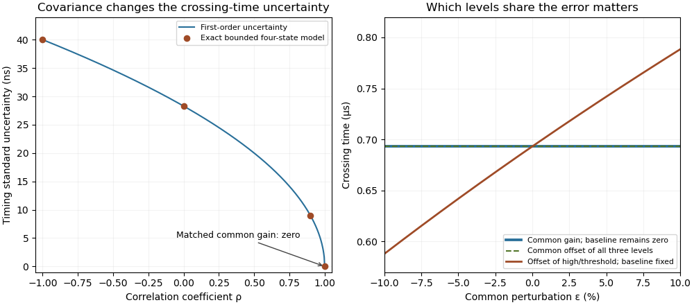
Covariance changes RC timing uncertainty, while gain and offset cancellation depend on the full measurement model
. Original calculation for a 1 V high level, 0.5 V threshold and 1 µs time constant. Exact four-state bounded-error checks are compared with first-order propagation. The right panel distinguishes common gain, a two-level offset with fixed baseline, and a common offset of all three levels. Its common perturbation sets gain or offset . No measured uncertainty data are used. Details.State-dependent gain in symmetric overlap measurements is a multiplicative response that changes with the optical radius-setting state. It can imitate the radius mismatch inferred from a symmetric log-overlap ratio. An acquisition order that cancels time drift does not remove a scale change tied to the state itself.
For positive overlap readings, supposewhere is the true logarithmic radius ratio, is a fixed state-specific gain and is shared logarithmic drift. Even after perfectly removing , the measured log-ratio isHere describes the known symmetric radius settings. The two unknowns and cannot be determined from this one ratio without further information. This is an identifiability problem, not merely a larger readout variance.
For an original matched-beam example, gives . A state-gain ratio instead produces . With , ignoring the gain difference givesapproximately 0.98379. The apparently small radius mismatch is entirely instrumental in this stipulated example. Repeating the same states more often reduces independent scatter without removing the state offset.
A reference-state transfer in overlap normalization can supply additional information. If a reference has known and the same state-gain ratio as the specimen measurement, its observed log-ratio estimates . Subtracting that log-ratio is justified only if the state response transfers. Changing optical power, detector operating point or aperture illumination between reference and specimen can break that assumption.
Another explicit model uses a simultaneous monitor with the same constant in both states. Then , and the state difference cancels the monitored gain. A separate optical-power monitor does not automatically satisfy this equation for an RF-amplifier gain change: verify which part of the measurement chain the monitor actually samples.
NIST's primary receiver apparatus uses variable attenuators, a beam splitter, a polarizer and single-mode-fibre coupling to match the incident modes, followed by electrical calibration.[ref]
Frequency response metrology for high-speed optical receivers by Paul D. Hale and others. PDF p. 1, Heterodyne measurements
Those controls motivate distinguishing an electronic gain change from an optical change in polarization, clipping or beam shape. The reference and monitor designs above are original diagnostic models, not procedures attributed to that paper.The covariance of differential spectral-calibration gains describes the joint errors of gain differences used in several spectral ratios. Let the calibration-error vector be with covariance , and form differences . ThenThis covariance identity is exact for the linear differences; no normal-distribution assumption is required. The first-order relation between gain differences and isotope stiffness ratios is given in separate spectral-calibration gains in isotope stiffness inference.[ref]
Guidelines for Evaluating and Expressing the Uncertainty of NIST Measurement Results by Barry N. Taylor and Chris E. Kuyatt. Appendix A, equation A-3, sensitivity and covariance propagation
For an original shared-reference model, take three gain errors , where is a common scale error and the are independent residual errors with variances . Two sample spectra are compared with the same reference spectrum:The common scale cancels, but the residual reference error remains in both differences:Cancellation of one common influence therefore does not establish independent comparisons.
Choose all three residual standard uncertainties as . Then , with correlation between the differences. Even a much larger common scale uncertainty cancels in this stipulated model. Each inferred log stiffness ratio has error approximately twice its gain difference. Averaging the two log-ratio estimates gives variance and standard uncertainty about . Incorrectly treating them as independent would give only .
This shared-reference floor in averaged isotope stiffness ratios matters when many sample spectra reuse one calibrated reference. Independent extra sample readings reduce their own errors, while a reference component shared by all comparisons remains. Assess covariance from the actual reference reuse, calibration drift and repeated acquisition protocol. The matrix calculation concerns multiplicative calibration errors; uncertain peak assignment, isotope composition and additive spectral offsets need their own contributions.
A maximum-exposure constraint in paired Raman acquisition bounds each detector frame so that a bright channel stays below saturation. For pump-on/off pairs with common per-frame cap , the total live exposures satisfyFor a fixed pair count and wall-clock budget, readout overhead in Raman exposure allocation leaves . Using the full budget is feasible only if ; otherwise one must change the pair count, shorten the acquisition or allow unused time.
Under the independent large-count shot-noise model, minimize . The feasible on-exposure interval isThe objective is strictly convex for positive on/off exposures. Its unconstrained optimum is ; clip that value to the feasible interval, retaining positive time in both states. This follows from the derivative changing sign once, rather than requiring a new unconstrained allocation rule.
For an original model, set , , , and . With six pairs, and the unconstrained on total exceeds its cap . The constrained choice is , , with . Five and seven pairs give approximately and respectively under the same model. Six is preferable among these three choices.
The integer frame-count choice under a Raman saturation limit must also include switching cadence, drift and read noise when relevant. The primary apparatus used 97 ms exposures to avoid detector saturation and 10 ms shuttered readout.[ref]
Femtosecond Broadband Stimulated Raman: A New Approach for High-Performance Vibrational Spectroscopy by David W. McCamant and others. Data Collection, exposure limit, S1/S2 shutter sequence and readout preceding equation 4
Those values motivate the stipulated numerical cap above; they are not universal detector specifications. A different optical flux or detector gain changes the usable exposure limit. Pinned article: Introduction to the OurBigBook Project
Welcome to the OurBigBook Project! Our goal is to create the perfect publishing platform for STEM subjects, and get university-level students to write the best free STEM tutorials ever.
Everyone is welcome to create an account and play with the site: ourbigbook.com/go/register. We belive that students themselves can write amazing tutorials, but teachers are welcome too. You can write about anything you want, it doesn't have to be STEM or even educational. Silly test content is very welcome and you won't be penalized in any way. Just keep it legal!
Intro to OurBigBook
. Source. We have two killer features:
- topics: topics group articles by different users with the same title, e.g. here is the topic for the "Fundamental Theorem of Calculus" ourbigbook.com/go/topic/fundamental-theorem-of-calculusArticles of different users are sorted by upvote within each article page. This feature is a bit like:
- a Wikipedia where each user can have their own version of each article
- a Q&A website like Stack Overflow, where multiple people can give their views on a given topic, and the best ones are sorted by upvote. Except you don't need to wait for someone to ask first, and any topic goes, no matter how narrow or broad
This feature makes it possible for readers to find better explanations of any topic created by other writers. And it allows writers to create an explanation in a place that readers might actually find it.
Figure 1. Screenshot of the "Derivative" topic page. View it live at: ourbigbook.com/go/topic/derivativeVideo 2. OurBigBook Web topics demo. Source. - local editing: you can store all your personal knowledge base content locally in a plaintext markup format that can be edited locally and published either:This way you can be sure that even if OurBigBook.com were to go down one day (which we have no plans to do as it is quite cheap to host!), your content will still be perfectly readable as a static site.
- to OurBigBook.com to get awesome multi-user features like topics and likes
- as HTML files to a static website, which you can host yourself for free on many external providers like GitHub Pages, and remain in full control

Figure 2. You can publish local OurBigBook lightweight markup files to either OurBigBook.com or as a static website.
Figure 3. Visual Studio Code extension installation.
Figure 5. . You can also edit articles on the Web editor without installing anything locally. Video 3. Edit locally and publish demo. Source. This shows editing OurBigBook Markup and publishing it using the Visual Studio Code extension. 
- Infinitely deep tables of contents:



All our software is open source and hosted at: github.com/ourbigbook/ourbigbook
Further documentation can be found at: docs.ourbigbook.com
Feel free to reach our to us for any help or suggestions: docs.ourbigbook.com/#contact