A gear contact-set consistency check verifies that a proposed solution satisfies force balance and the unilateral contact conditions used to define a gear mesh active-contact set. Solving an equation for selected contacts is insufficient if an omitted tooth should be loaded or an included tooth would require tension.

For the model $F_j=k_j\max (\delta -e_j,0)$, choose a trial active set $\mathcal{A}$ and solveThe check then requires positive $k_j(\delta -e_j)$ for included pairs and $\delta \le e_j$ for excluded pairs. Recomputing every contact with the unilateral law gives the force residualA consistent exact solution has $r_F=0$ together with the inclusion inequalities.

An original example has stiffnesses $100,50,150N/\mu \mathrm{m}$ and gaps $0,2,5\mu \mathrm{m}$. At $F_{\mathrm{applied}}=900\mathrm{N}$, a trial set containing only the first two pairs gives $\delta =20/3\mu \mathrm{m}$. It balances those selected forces but exceeds the third gap by $5/3\mu \mathrm{m}$. The omitted contact would carry $250\mathrm{N}$, giving $r_F=250\mathrm{N}$. Including all three gives the consistent approach $35/6\mu \mathrm{m}$.

Conversely, including all three at applied load $500\mathrm{N}$ gives the un-clipped solution $\delta =4.5\mu \mathrm{m}$ and a third force $-75\mathrm{N}$. Rejecting that tensile contact and solving with the first two gives $\delta =4\mu \mathrm{m}$ and forces $400,100,0\mathrm{N}$.

Numerical tolerances should keep their units and roles clear. A displacement tolerance near a gear tooth engagement threshold is not the same quantity as a force-residual tolerance. At an exact zero-force touch, either a geometric-touch flag or the positive-force active convention may be useful, but the reported convention must be stated. The one-sided gear mesh tangent stiffness can differ across that boundary.

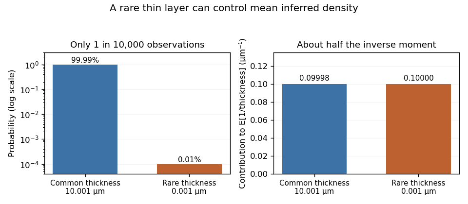
Primary dynamic gear analysis couples tooth stiffness and calculated loads as contact position changes.^[ref] The scalar check above validates internal consistency of its quasistatic model; it does not establish that the model includes every deformation or dynamic effect in a real mesh.

Tail-model dependence of inferred density uncertainty is the sensitivity of a density estimate's distribution to the assumed probability of very small positive thicknesses. For $\rho =K/\delta$ with fixed $K=M/A>0$, a tiny thickness has disproportionate influence through $1/\delta$. The main body of a thickness histogram can look stable while the inferred mean or variance remains model-dependent.

A gamma distribution and a lognormal distribution provide useful explicit models. NIST specifies their density functions and parameter conventions.^[ref] At mean thickness $d$ and coefficient of variation $c$, the gamma model has shape $a=1/c^2$ and givesThe lognormal model gives $(1+c^2)/d$. The two agree closely for small $c$, but that agreement concerns those model families, not every positive distribution with a similar spread.

An original rare-event example makes the limitation explicit. Let thickness be $0.001$ micrometres with probability $0.0001$ and $10.001$ micrometres otherwise. Mean thickness is exactly 10 micrometres and its standard deviation is approximately 0.10 micrometres, about 1% of the mean. Nevertheless,nearly twice the reciprocal of mean thickness. The rare component supplies about half the inverse moment. These are deliberately constructed model values, not measured polymer-layer dimensions.

Rare-thickness leverage on inverse moments can escape an apparently reassuring sample. With 1,000 independent thickness observations, the chance of seeing none of that rare component is $(0.9999{)}^{1000}\approx 0.905$. A finite simulation or a smooth fit to common observations need not validate the unobserved lower tail.

A useful experiment investigates whether dimensional resolution, specimen geometry or physical constraints rule out such near-zero layers. Report sensitivity to defensible alternative lower-tail models or measured lower bounds. Choosing a positive distribution guarantees positive thickness, but does not establish that its inverse moments describe the measurement process.

A time-dependent decay-rate envelope bounds a nonnegative signal using a lower bound on its instantaneous decay rate. If $P$ is absolutely continuous on finite intervals, $P(b)\le A$ and $P^{\prime }\le -k(t)P$ almost everywhere for locally integrable $k(t)\ge 0$, thenThe differential inequality for an exponential tail envelope article proves this comparison using an integrating factor and gives a piecewise-constant example. A strictly positive constant lower bound on $k$ gives exponential decay, but a positive rate at every instant need not supply such a lower bound.

An original example takes $k(t)=\alpha /(t-b+t_0)$ with $t_0>0$ and $\alpha >0$. Its integrated rate is logarithmic, soThis power-law tail from a decaying rate envelope tends to zero for every positive $\alpha$. Its envelope energy is nevertheless finite only when $\alpha >1$, in which caseFor original chosen $A=0.20\mathrm{W}$, $t_0=5\mathrm{ns}$ and $\alpha =2$, the allowance is $1.0\mathrm{nJ}$. After a further $45\mathrm{ns}$ it is at most $0.10\mathrm{nJ}$. The remaining energy decreases algebraically rather than exponentially.

At $\alpha =1$ the integrated envelope diverges logarithmically despite its power tending to zero. This does not prove that every signal below it has infinite energy; it means these assumptions alone supply no finite all-time energy bound. Taking the envelope itself gives a mathematical counterexample to the claim that pointwise decay implies integrable energy.

An experimental rate law therefore needs both temporal validity and an integrability check before it bounds missed optical energy. A measured detector tail is not automatically the true power profile; NIST's primary calibration procedure measures the receiver response separately.^[ref] The power-law example is an independent comparison model, not a reported tail law of that apparatus.

The joint exponential moment in overlap correction is the expected value $\mathbb{E}[\exp (d-\hat{v}/2)]$ that controls the mean of a variance-corrected overlap estimate. It retains the dependence between a logarithmic reading error $d$ and its estimated variance $\hat{v}$. Separate marginal distributions do not determine this expectation.

For $\hat{\gamma }=\gamma e^d$ and $\tilde{\gamma }=\hat{\gamma }{e}^{-\hat{v}/2}$,An original multivariate Gaussian integral evaluates a useful family exactly. Let $Z\sim N(0,I_n)$, $d=a^{\mathsf{T}}Z$ and $\hat{v}=c+Z^{\mathsf{T}}BZ$, with $c\ge 0$ and $B$ a symmetric positive semidefinite matrix. Completing the square givesIndeed, combining the Gaussian density with the correction changes its precision matrix to $I_n+B$ and shifts its center to $(I_n+B{)}^{-1}a$. Integration gives the determinant factor. Positive semidefiniteness keeps the variance estimate nonnegative and the integral finite. This is a quadratic Gaussian overlap correction model, not a receiver specification.

The log-error variance is $a^{\mathsf{T}}a$, while $\mathbb{E}[\hat{v}]=c+\mathrm{tr}B$. Equality of those quantities makes the variance estimate unbiased; it does not make the corrected overlap unbiased.

For a concrete two-dimensional example, take $a=(1,0{)}^{\mathsf{T}}$ and $c=0$. Choosing $B=\mathrm{diag}(1,0)$ uses the same normal component in both the reading and variance estimate, giving $e^{1/4}/\sqrt{2}\approx 0.90794$. Choosing $B=\mathrm{diag}(0,1)$ uses an independent component, giving $e^{1/2}/\sqrt{2}\approx 1.16582$. Both variance estimates have the same chi-squared distribution and mean one. Their different joint relationships to the reading reverse the direction of the remaining bias.

In a measurement implementation, preserve which calibration residuals and normalization records are shared. JCGM 101 distinguishes joint input assignment from numerical propagation and discusses multivariate Gaussian inputs and prior uncertainty calculations.^[ref] A Monte Carlo method can reproduce the integral for a specified joint model; independently resampling shared records would test another model. Compare simulated means with this exact family before interpreting numerical convergence as evidence about a physical receiver.

Third-order correlation brightness weighting is the way bright shots contribute disproportionately to an averaged nonlinear correlation trace. A normalized average trace is a weighted mean of shot-normalized shapes, with weights set by their central correlation signals rather than by how often the shots occur.

Let a nonnegative, background-corrected third-order trace on shot $j$ be $A_j(\tau )$. Define its central signal $B_j=A_j(0)>0$ and normalized shape $r_j(\tau )=A_j(\tau )/B_j$. Then the experimentally distinct averages areand the equal-shot mean $R_{\mathrm{shot}}(\tau )=N^{-1}{\sum }_j{r}_j(\tau )$. The nonnegative $w_j$ sum to one, but are equal only when the $B_j$ are equal. Here “central” denotes the specified zero-delay signal, not whichever noisy sample happens to be the largest.

For identical pulse shapes multiplied by intensity factors $K_j$, the ideal integral $A_j(\tau )=\int I_j^2(t)I_j(t+\tau )dt$ scales as $K_j^3$. The primary correlator implements this three-intensity-factor gate using second-harmonic generation followed by sum-frequency generation.^[ref] If shapes change, $B_j$ can depend on duration and overlap as well as brightness, so pulse energy alone need not determine the weight.

An original two-class example has equally frequent classes with $(B,r)=(1,0.01)$ and $(8,0.10)$ at one chosen delay. Their equal-shot mean ratio is $0.055$, but the normalized summed trace givesThe bright class supplies eight ninths of the central signal despite representing only half the shots. Neither result is an arithmetic mistake: they estimate different summaries of the stipulated ensemble.

For an ensemble with finite moments and $\mathbb{E}[B]>0$, the distinction can be expressed exactly through covariance:Unchanged normalized shape makes the covariance zero, even with large brightness fluctuations. Shape–brightness dependence can make it nonzero; cubic intensity-noise bias in pulse correlation alone does not prove a contrast change.

A shot-resolved pulse-contrast estimator needs synchronized intensity information and a stated selection rule. Thresholding weak shots or dividing by a noisy central signal can introduce further selection and ratio errors. Report whether normalization occurred before or after averaging, retain detector baseline subtraction, and test readout linearity. A smooth averaged trace is not a representative single shot unless those assumptions are justified.

A floating-pinion affine uncertainty bound evaluates the minimum contact-compression margin when the approach and imbalance depend linearly plus a constant on bounded shared parameters. It gives an exact result for a box of uncertainty variables, while preserving the dependence those variables induce between physical quantities.

In the correlated floating-pinion uncertainty set, supposeAll uncertainty vectors in this box are assumed admissible. For the linear two-contact model, the floating-pinion robust contact margin is the infimum of $\delta -|b|$ over that box.

First resolve the absolute value:For any affine expression $q_0+{\sum }_j{q}_j{u}_j$, its minimum is $q_0-{\sum }_j{\rho }_j|q_j|$: choose each bounded variable with the sign opposing its coefficient. Applying this rule to the two branches givesThe branches can attain their minima at different parameter vectors. Taking the smaller of their independently attainable minima is valid; requiring both minima to occur at one vector would impose an unnecessary condition.

For an original example in micrometres, letThe two branch minima are $4.5-0.1-0.3=4.1$ and $5.5-0.3-0.1=5.1$, so $M_{\mathrm{rob}}=4.1\mu \mathrm{m}$. The first is attained at $(u_1,u_2)=(-1,-1)$. Treating the separate physical ranges independently instead gives ${\delta }_L=4.7$ and $\max |b|=0.8$, hence a looser $3.9\mu \mathrm{m}$ bound. A motion amplitude $4.0\mu \mathrm{m}$ leaves guaranteed compression $0.1\mu \mathrm{m}$ in the shared-variable model.

The result is exact for the stated box and affine model. Additional constraints can make it conservative; nonlinear parameter dependence or opening of a contact can invalidate the model itself. A floating-pinion ellipsoidal uncertainty bound addresses a different set shape, and a statistical covariance matrix alone does not certify a hard bound.

NASA's face-gear report supplies the physical motivation for examining mounting freedom and load sharing, not an experimental validation of these chosen uncertainty coefficients.^[ref] A valid guarantee requires defensible parameter bounds and the appropriate floating-pinion contact-loss check.

Batch-matched blank weighting applies background corrections in the same proportions as the specimen results they correct. It concerns the definition of the target mean as well as the precision of the blank measurements. An experiment on blank-corrected carbon recovery in polymer tests can have different backgrounds across preparation batches even when every batch follows the same nominal procedure.

For an original additive model, let $T_b={\mu }_b+{\beta }_b+{ϵ}_b$ be a batch specimen mean and $B_b={\beta }_b+{\eta }_b$ its blank mean, with zero-mean measurement errors. The desired scientific target is $\mu ={\sum }_b{w}_b{\mu }_b$, where ${\sum }_b{w}_b=1$. If specimen means use $w_b$ but blanks use different weights $a_b$, the estimatorhas bias ${\sum }_b(w_b-a_b){\beta }_b$. Matching $a_b=w_b$ removes that bias for arbitrary batch backgrounds in this model. Pooling can remain unbiased under an additional justified common-background assumption, but that is a different model.

For stipulated backgrounds 2 and 8 mg and target weights 0.75 and 0.25, the relevant correction is 3.5 mg. An equally weighted pooled correction is 5 mg and biases the net mean downward by 1.5 mg. Dividing that net result by a fixed 50 mg initial-carbon amount shifts the recovery fraction by $-1.5/50=-0.03$, or three percentage points. These are constructed examples, not OECD test results.

With independent specimen and blank estimates, variance propagation gives $\mathrm{Var}(\hat{\mu })={\sum }_b{w}_b^2\mathrm{Var}(T_b)+{\sum }_b{a}_b^2\mathrm{Var}(B_b)$. Common reference measurements require covariance terms as well.^[ref] Changing weights to reduce variance can change the target or introduce bias; it is not automatically an improvement.

Transporting blank corrections between batches requires evidence that their backgrounds are exchangeable for the intended correction. OECD's general principle already cautions that endogenous activity with a test chemical need not match the inoculum control.^[ref] Matching batch weights repairs an aggregation error; it does not establish chemical additivity. State the target population, batch labels, normalization amounts and pooling assumptions before deciding which measurements share a correction.

Bipes is a taxonomic genus of burrowing amphisbaenians distinguished by retaining external forelimbs despite an elongated body and absence of external hindlimbs. It is an informative comparison with other amphisbaenians, which lack external limbs: external appearance alone does not reveal how much internal anatomy remains.^[ref]

In a 2019 anatomical study, investigators used iodine-enhanced computed tomography to distinguish soft tissues and reconstruct shoulder muscles as well as bones. Bipes retained an almost complete shoulder girdle, while other sampled amphisbaenians had much more reduced bony structures. Nevertheless, all sampled amphisbaenian forms retained the full set of 17 shoulder muscles, sometimes fused or rearranged. Muscle attachment could shift from bone to surrounding soft tissue.^[ref]

The result challenges a tempting shortcut: losing a visible limb does not necessarily delete all its associated muscles at once. Bipes supplies the limbed comparison that helps reveal which internal components have persisted or changed during the evolution of the burrowing body form.

Acquisition-time sensitivity to tail-model parameters measures how an inferred recording extension changes when the assumed optical tail changes. In the positive-duration branch of acquisition duration from an exponential tail-energy tolerance, writeHere $A$ bounds the initial tail power, $\tau$ is its decay time and $\epsilon$ the tolerated missed energy. Their first-order relative effects areThese logarithmic condition numbers of a tail-acquisition requirement distinguish a fractional amplitude error from a fractional decay-time error. For a stringent tolerance with large $\ell$, decay-time sensitivity stays near unity while amplitude sensitivity decreases.

For an original example, take $A=0.20\mathrm{W}$, $\tau =20\mathrm{ns}$ and $\epsilon =0.040\mathrm{nJ}$. Then $A\tau /\epsilon =100$ and $L\approx 92.10\mathrm{ns}$. Let the independent standard uncertainties of $A$ and $\tau$ be $10\%$ and $5\%$, with the tolerance fixed. The amplitude contribution to $u(L)$ is $2.00\mathrm{ns}$; the decay-time contribution is $(1+\log 100)\times 1\mathrm{ns}\approx 5.605\mathrm{ns}$. Adding their variances gives $u(L)\approx 5.95\mathrm{ns}$, about $6.46\%$.

Correlated fitted parameters require covariance terms in this propagation.^[ref] A standard uncertainty is not a guaranteed recording margin: a worst-case requirement needs a justified allowed parameter set, as in the parent article. The zero-duration boundary is also outside this smooth positive-branch calculation.

Physically, these parameters must describe the unrecorded optical power, not merely an electrical detector tail. NIST separately measured the detector/cable/oscilloscope response before correcting pulse measurements.^[ref] A precise fit to the wrong response component does not justify the optical envelope or its acquisition-time bound.

Dependent variance correction in heterodyne normalization occurs when an overlap reading and the estimated logarithmic variance used to correct it share random information. Correcting the reading is then a joint nonlinear calculation; multiplying separately averaged correction factors can give the wrong answer, even when the variance estimate is unbiased.

Write $\hat{\gamma }=\gamma e^d$ and $\tilde{\gamma }=\hat{\gamma }{e}^{-\hat{v}/2}$, with $d$ a centered normal random variable of variance $v$. The exact mean ratio isThe joint exponential moment in overlap correction cannot generally be replaced by $\mathbb{E}[e^d]\mathbb{E}[e^{-\hat{v}/2}]$. That factorization requires independence. JCGM 101 treats a measurement function of jointly distributed inputs and distinguishes choosing that joint model from propagating it.^[ref]

An original counterexample takes $\hat{v}=d^2$. This estimate is nonnegative and has expected value $v$, because the log-error mean is assumed known to be zero. It is completely dependent on the reading. It is a mathematical stress test, not a recommended way to estimate receiver noise from one observation.

Completing the square in a Gaussian integral givesSetting $a=t=1$ therefore yieldsAt stipulated $v=1$, the ratio is $e^{1/4}/\sqrt{2}\approx 0.90794$. An unbiased variance estimate has left a downward mean shift. The independence-based upward-shift argument in uncertain variance in heterodyne lognormal bias correction does not apply.

For comparison, let $d^{\prime }$ be an independent copy and use $\hat{v}=(d^{\prime }{)}^2$. The variance estimate has exactly the same marginal distribution, but the mean ratio becomes $e^{v/2}/\sqrt{1+v}$, approximately 1.16582 at $v=1$. Changing only the dependence reverses the direction of the residual bias. Both are illustrative probability models, not measured optical noise levels.

In a physical analysis, record which calibration records, fitted residuals and normalization readings are reused. A Monte Carlo method must reproduce those shared random inputs rather than independently drawing a new variance estimate wherever the formula uses it. An independent calibration sample simplifies some dependencies but can introduce drift between calibration and measurement. Neither strategy replaces checks on heterodyne RF-to-DC gain transfer check or stable optical alignment; the probability model describes residual uncertainty after those measurement paths have been specified.

The time above threshold for an RC-filtered rectangular pulse is the separation of its rising and falling threshold crossings, rather than the applied pulse duration. In the relaxed first-order model, put $a=V_{\mathrm{th}}/V_0$ with $0<a<1$ and $T>T_{\min }=-\tau \log (1-a)$. The parent crossing calculation givesThis excludes comparator propagation dynamics and uses the same threshold on both edges. A Schmitt trigger with unequal switching thresholds needs a different formula.

The positive-width relation can be inverted exactly:Its derivative is $dW/dT=1/(1-e^{-T/\tau })>1$. Thus a measured positive $W$ determines a unique input duration under the stated model. A zero-width observation does not: all rejected durations $T\le T_{\min }$ have that same outcome.

For an original example, take $a=0.25$, $\tau =1\mu \mathrm{s}$ and $T=2\mu \mathrm{s}$. The output remains above threshold for about $2.9532\mu \mathrm{s}$, longer than the input pulse because of its decaying tail. Substitution into the inverse relation recovers $2\mu \mathrm{s}$.

For long pulses, $W-T$ tends to $\tau \log [(1-a)/a]$. It is positive below a half-height threshold and negative above one. At exactly half height, $W<T$ for every finite accepted pulse, with the difference tending to zero for long pulses. Consequently a measured above-threshold width cannot be equated to the input width without the threshold and filter model.

A pulse-generator/oscilloscope comparison can record both widths while varying threshold. The measured RC decay should be checked independently, using the natural-response method in the primary MIT laboratory.^[ref] Initial residual charge, hysteresis, and different rising/falling comparator delays alter the observation; the algebra above only inverts the ideal capacitor waveform.

Threshold timing sensitivity of an RC step response measures how a crossing time changes when the absolute threshold or signal height changes. For a relaxed step response $v(t)=V_0(1-e^{-t/\tau })$, with $0<V_{\mathrm{th}}<V_0$, the rising crossing isHolding the other inputs fixed givesA threshold approaching the step height encounters a flatter part of the exponential response, making the first sensitivity large.

For an original timing estimate, choose $V_0=2\mathrm{V}$, $\tau =0.5\mu \mathrm{s}$, and effective small threshold-noise standard deviation $4\mathrm{mV}$. At $V_{\mathrm{th}}=0.4\mathrm{V}$, local linear propagation gives timing standard deviation about $1.25\mathrm{ns}$. At $1.9\mathrm{V}$, it gives about $20\mathrm{ns}$. The latter threshold also needs a longer input pulse to be reached at all, as shown in threshold-crossing time of a finite rectangular pulse through an RC load.

The two voltage sensitivities can cancel under a different measurement calibration model. If the threshold is set to a fixed fraction $a$ of the same varying height, $d{V}_{\mathrm{th}}=ad{V}_0$ and $V_{\mathrm{th}}=a{V}_0$, their contributions sum to zero. The crossing becomes $-\tau \log (1-a)$, independent of amplitude in this ideal model. Such correlated threshold and amplitude errors in RC timing must retain covariance rather than add two independent voltage uncertainties.^[ref]

The local noise rule also follows from dividing a small voltage perturbation by the crossing slope $(V_0-V_{\mathrm{th}})/\tau$. It assumes a well-defined nearby crossing and sufficiently small perturbations; it does not describe multiple noise crossings, comparator switching dynamics, or a pulse ending before the threshold. A bench test can compare controlled threshold shifts with oscilloscope crossing times while holding the actual step height and initial state fixed.

RC pulse-width discrimination converts an input-duration test into a threshold observation on an RC circuit. For a relaxed first-order load with time constant $\tau >0$, a positive rectangular input of height $V_0$ and duration $T$ reaches peak output $V_0(1-e^{-T/\tau })$. An ideal electronic comparator has a nonzero interval above fixed threshold $0<V_{\mathrm{th}}<V_0$ precisely whenEquality only touches the threshold at the peak. The parent threshold-crossing time of a finite rectangular pulse through an RC load derives the full response and the rejected-pulse boundary.

This is a duration discriminator only while the input height is controlled. At a fixed duration, the same condition isA larger input can pass the threshold even when a smaller pulse of exactly the same duration fails. The minimum accepted duration decreases with height, with derivative $-\tau V_{\mathrm{th}}/[V_0(V_0-V_{\mathrm{th}})]$.

For an original example, choose $\tau =2\mu \mathrm{s}$, $V_{\mathrm{th}}=0.40\mathrm{V}$, and $T=1\mu \mathrm{s}$. The minimum height for a nonzero comparator interval is about $1.0166\mathrm{V}$. A $0.8\mathrm{V}$ pulse peaks at about $0.3148\mathrm{V}$ and is rejected; a $1.2\mathrm{V}$ pulse peaks at about $0.4722\mathrm{V}$ and is accepted. Treating this observation as a width-only decision would conflate two different inputs.

A pulse-generator experiment therefore sweeps width at a recorded height and threshold, measures the actual capacitor waveform on an oscilloscope, and allows the initial state to relax. A residual baseline in RC pulse-width discrimination changes the next pulse's peak and invalidates the relaxed-state formula. Probe and comparator input capacitance also belong in the effective time constant. The natural-decay apparatus in MIT's RC laboratory supplies a direct component-level check of that time constant.^[ref] Comparator propagation delay and hysteresis are additional dynamics, not part of the ideal RC acceptance inequality.

A tie-line phase-fraction fit estimates how much of each liquid phase is needed to reproduce an overall composition from specified liquid-liquid tie line endpoints. If ${\mathbf{x}}^{\alpha },{\mathbf{x}}^{\beta }$ are endpoint mole fraction vectors and $\lambda$ is the mole-based phase fraction of phase $\beta$, the mass balance predictsThe endpoints must be supplied by equilibrium measurements or a suitable thermodynamic model; fitting $\lambda$ does not establish that an arbitrary pair of compositions is an equilibrium tie line.^[ref]

For a ternary liquid-liquid tie line, use two independent composition coordinates, such as the first two mole fractions, since the third is fixed by their sum. Let $\mathbf{y}$ be these two measured coordinates, $\mathbf{a}$ the corresponding phase-$\alpha$ coordinates, $\mathbf{d}$ the difference between phase-$\beta$ and phase-$\alpha$ coordinates, and $\Sigma$ a positive-definite covariance matrix for $\mathbf{y}$. With exact endpoints, generalized least squares minimizesDifferentiation yields the unconstrained estimateThe second expression imposes the physical bounds. It follows because $J$ is a convex quadratic when the endpoints differ in the measured coordinates. The ternary tie-line consistency residual then records the remaining failure of the mass balance.

For an original hypothetical example, take endpoint compositions $(0.60,0.30,0.10)$ and $(0.20,0.40,0.40)$, with overall measurement $(0.470,0.325,0.205)$. Suppose the first two measured mole fractions have independent standard measurement uncertainties $0.010$ and $0.005$, so $\Sigma =\mathrm{diag}(0.010^2,0.005^2)$. ThenThe predicted composition is $(0.476,0.331,0.193)$, giving residual $(-0.006,-0.006,0.012)$. The separate first- and second-component balances would suggest $0.325$ and $0.250$; the fit combines them according to their stated measurement uncertainties, rather than averaging those two numbers without regard to precision.

With Gaussian composition errors, fixed endpoints and an interior unconstrained fit, the tie-line phase-fraction uncertainty follows directly from the linear estimator:for this example. Endpoint uncertainty, a fit on a boundary, or a nearly vanishing endpoint difference needs additional treatment. In particular, all three normalized mole fractions must not be treated as independent observations with an invertible three-coordinate covariance matrix: their exact closure creates dependence. A small fitted residual is evidence of consistency with the specified mass balance and error model, not a substitute for testing chemical potential equality or phase stability.

Inversion of a symmetric Gaussian overlap log-ratio recovers a radius ratio from two positive overlap-efficiency measurements made at known symmetric radius settings. It applies to the one-parameter model of symmetric beam-radius perturbation for overlap branch selection, with one shared response scale and fixed remaining mode properties.

Let $h=\log q>0$, $D_h=\log (V_{+}/V_{-})$ and $u=\log \rho$, where $\rho =w_2/w_1$. Since the symmetric log-overlap ratio satisfies $D_h=-4\mathrm{artanh}(\tanh h\tanh u)$, defineThenA finite positive radius ratio exists exactly when $|z|<1$, equivalently $|D_h|<4h$. The strictly decreasing forward relation makes the solution unique inside this interval. Equality corresponds only to a limiting zero or infinite radius ratio; an out-of-range noisy measurement has no finite solution in this ideal model.

For an original example, $q=2$ and $D_h=\log (289/64)$ give $\tanh h=0.6$ and $z=-0.6$, hence $\rho =1/2$. If the known first radius is $100\mu \mathrm{m}$, the inferred second radius is $50\mu \mathrm{m}$. The nuisance scale is unnecessary for that inversion. Once $\rho$ is obtained, one can reconstruct it as $A=V_{+}{\cosh }^2(u+h)$, but two fitted readings alone do not validate the Gaussian optical model.

The inverse sensitivity isFor small errors, relative radius uncertainty is approximately $u(\rho )/\rho \simeq |du/d{D}_h|u(D_h)$. At the worked point the derivative is $-17/30$; stipulated $u(D_h)=0.02$ gives about 1.13% relative radius uncertainty, before including uncertainty in the setting $h$ or the reference radius.

Near the allowed interval's edges, the inverse becomes highly sensitive. Boundary-sensitive Gaussian overlap inversion needs an uncertainty model that respects the nonlinear transformation; clipping an out-of-range value to a convenient radius does not supply the missing information. The GUM distinguishes local uncertainty propagation from cases requiring higher-order treatment.^[ref]

The apparatus must implement a radius change without unintended displacement, polarization or wavefront changes. NIST's physical heterodyne receiver experiment used mode and polarization control and separate electrical corrections.^[ref] Those controls motivate checks on the inversion assumptions; the paper is not a report of the particular symmetric-radius example derived here.

Symmetric-overlap normalization drift is a time-dependent change in the multiplicative scale of two overlap readings. The symmetric log-overlap ratio cancels one shared scale, but sequential settings need not experience that same scale.

Let the stable optical contributions at the two radius settings be $F_{+}$ and $F_{-}$, and letwhere $a(t)=\log A(t)$. The ideal log-ratio is $D_0=F_{+}-F_{-}$. A positive-setting reading at time 0 followed by a negative-setting reading at time $\Delta$ instead gives $D_{\mathrm{obs}}=D_0+a(0)-a(\Delta )$. A drift in normalization can therefore mimic a signed radius mismatch.

An original four-reading design uses settings $+,-,-,+$ at equally spaced times $0,\Delta ,2\Delta ,3\Delta$. FormThe scale contribution vanishes exactly when $a(t)$ is linear in time: both settings have the same mean observation time. This cancels linear drift in logarithmic scale, not arbitrary drift in every measured quantity.

If $a(t)=a_0+bt+c{t}^2$, the remaining drift contribution is $2c{\Delta }^2$. For stipulated $D_0=0.05$, $b=0.02$ per time unit and $\Delta =1$, a simple two-reading comparison gives 0.03 under purely linear log-drift, while the four-reading design gives 0.05. Adding $c=0.003$ per squared time unit changes the latter to 0.056. These are analytical timing examples, not measurements from a beam experiment.

With independent equal log-readout variance ${\sigma }^2$, the four-reading estimator has variance ${\sigma }^2$, because it combines four coefficients of magnitude one half. A single two-reading difference has variance $2{\sigma }^2$ at half the acquisition count. Correlated noise and longer acquisition time can change the practical tradeoff.

State-dependent gain in symmetric overlap measurements does not cancel through this ordering. If the scale changes systematically with the radius-setting state, it remains confounded with $F_{+}-F_{-}$. The optical mismatch must also remain stable over the sequence; a changing beam is not merely an electronic scale drift.

NIST controlled mode and polarization matching while calibrating the receiver's electrical response.^[ref] The ordering above is an original drift-control calculation, not an attributed NIST procedure. Test its assumptions with timing records, repeated sequences and independent monitoring before feeding the resulting ratio into the radius inversion.

An amphisbaenian is a member of Amphisbaenia, a lineage of predominantly burrowing Squamata. The elongated body often has rings of scales, small eyes and a skull specialized for moving through soil. Most species lack external limbs, but Bipes retains forelimbs. Their wormlike appearance does not make them Annelida, and a limbless body does not make them snakes.

Their evolutionary relationships illustrate the problem of convergent evolution. Burrowing can favor similar reductions and skull modifications in separate reptile lineages, making an anatomy-only grouping misleading. An integrated 2015 study compared morphological characters, molecular sequences and fossil taxa, and recovered amphisbaenians with lacertids in Lacertoidea. Including DNA allowed the investigators to test similarities that might instead reflect similar modes of life.^[ref]

The example shows why a shared loss of limbs must be interpreted on a phylogenetic tree, alongside other evidence, before it is treated as evidence of close ancestry.

A skink is a lizard in the family Scincidae, within Squamata. The family contains a wide range of body forms, from animals with four well-developed limbs to elongated forms with strongly reduced limbs or none externally visible. A long, legless body therefore does not establish that a reptile is a snake.^[ref]

A 2023 comparative dataset classified $22.8\%$ of its skink species as having reduced or absent limbs, using limb proportions relative to snout-to-vent length. This makes the comparison measurable: a short absolute leg length in a tiny animal is different from a short leg relative to the animal's body. Placing those measurements on a phylogenetic tree permits tests of repeated evolutionary changes instead of treating every similar body shape as one inherited event.^[ref]

Reproduction is diverse as well. Some skinks lay eggs and others give birth to live young. In the same dataset, about one third of the species with known reproductive mode were live-bearing; that qualification matters because unknown cases were excluded. A family name captures ancestry without requiring every member to share one body plan or reproductive mode.^[ref]

Lacertoidea is a branch of Squamata containing Lacertidae, Teiidae, Gymnophthalmidae and amphisbaenians. It groups lineages by common ancestry, despite striking differences in their visible bodies. In particular, a burrowing, nearly limbless amphisbaenian can be more closely related to a normally limbed member of Lacertidae than superficial resemblance to a snake suggests.^[ref]

This grouping is a useful test of convergent evolution. Imagine recording only whether an animal has external legs: many otherwise unrelated burrowing forms would receive the same score. Recording hundreds of anatomical characters and comparing many genes supplies additional, partly independent evidence. The 2015 integrated analysis used 691 morphological characters and 46 genes, and included fossils as well as living species. Its combined analyses recovered Lacertoidea, while some deeper relationships depended on uncertain placements of fossil taxa.^[ref]

Moment conditions for baseline-drift cancellation specify which polynomial backgrounds a linear measurement removes. Let readings at known times $t_i$ enter the corrected pulse estimate as $\hat{U}={\sum }_i{a}_i{x}_i$, with the integration/calibration units included in $a_i$. A background $b(t)={\sum }_{q=0}^p{c}_q{t}^q$ contributes nothing wheneverSubstitution gives this result directly. The zeroth condition removes a common offset; the first additionally removes linear drift. These conditions concern the actual weights and times, not only the number of background samples.

An original one-bin signal model measures a pulse at $t=0$, with uncontaminated reference samples at $-h$ and $h$. UseThe weights sum to zero and have zero first time moment. Constant and linear backgrounds cancel exactly, but a quadratic background $c_2{t}^2$ leaves bias $-\Delta t{c}_2{h}^2$. With chosen $h=2\mu \mathrm{s}$, $\Delta t=1\mu \mathrm{s}$ and $c_2=0.05mW/\mu {\mathrm{s}}^2$, the bias is $-0.20\mathrm{nJ}$. Here the pulse is stipulated to occupy the central bin; the formula is not a universal integral estimator for an arbitrary waveform.

Cancellation has a noise cost of polynomial baseline cancellation. For independent equal-variance reading errors ${\sigma }^2$, the chosen estimate has variance $(3/2)\Delta t^2{\sigma }^2$, even though its constant and linear bias terms vanish. General correlations use ${\mathbf{a}}^{T}C\mathbf{a}$ instead.^[ref]

NIST's historical pulse-energy apparatus used before/after baselines for background and thermal-drift compensation.^[ref] The polynomial test above is an original general analysis. Pulse contamination in a reference, uncertain timing or drift outside the assumed polynomial family can leave a residual even when the nominal algebraic conditions hold.