Use consistent units for the Gibbs free energy:Then $\Delta G^{\circ }=-RT\ln K$ givesThis is a dimensionless thermodynamic equilibrium constant defined through activities. For an ideal dilute $1:1$ association, the numerical concentration association constant is about $4.53\times 10^3{\mathrm{M}}^{-1}$ when concentrations use the $1\mathrm{M}$ standard state. Both favourable enthalpy and positive entropy favour association here; association need not always have a negative entropy change because solvent release can outweigh the loss of translational freedom.

Increasing the angular acceptance can collect higher spatial frequencies, but rays at large angles and away from the optical axis are harder to bring to the same focus. Spherical aberration, coma, astigmatism and field curvature can degrade contrast across a large exposure field. The depth of focus also decreases approximately as $\lambda /{\mathrm{NA}}^2$, making wafer height errors more important. A larger geometrical aperture is therefore not automatically better over the whole wafer field.

Immersion lithography raises $\mathrm{NA}=n\sin \theta$ by increasing the refractive index of the medium between the final lens and wafer. A suitable UV-transparent liquid permits a larger numerical aperture without increasing the ray angle by the same factor, easing the purely geometrical demand on the lens. Lens design and focus control remain necessary; immersion does not abolish aberrations. The liquid must also be compatible with the resist and free of bubbles and contamination, and absorption at $193\mathrm{nm}$ must be low.

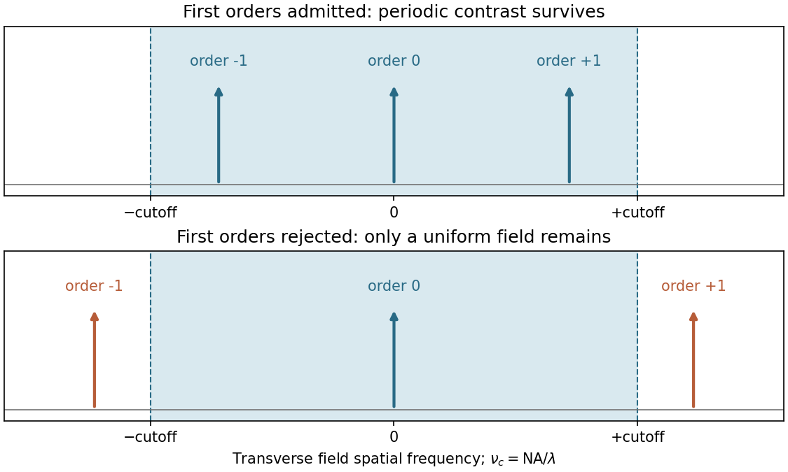
The projection lens maps the mask's angular spectrum into its back focal plane: within scalar Fourier optics this is the Fraunhofer diffraction or spatial-Fourier plane. A periodic mask produces discrete diffraction orders, separated by $1/P$ in object-side spatial frequency after accounting for projection magnification. The finite numerical aperture bounds the transverse wave vectors admitted by the lens, so the pupil is a spatial-frequency filter.

For an ideal on-axis coherent system,A second Fourier transformation forms the image, and the recorded intensity is $|U_{\mathrm{image}}{|}^2$. If only the zero order passes, the field is uniform and the line pattern disappears. Passing zero and first orders restores a periodic modulation; passing more orders sharpens the edges. Thus the loss of fine structure is explained by rejected diffraction orders, not by a geometrical inability to draw narrow lines. The field-transfer cutoff differs from the twice-as-large incoherent intensity-transfer cutoff.^[ref]

Take the ArF wavelength as $\lambda =193\mathrm{nm}$ and assume an on-axis coherent illuminator. A grating of period $P$ has diffraction orders with transverse spatial frequencies $m/P$. To reproduce amplitude modulation, the pupil must pass the zero order and at least the first spatial-frequency components. For symmetric on-axis illumination this requires $1/P<\mathrm{NA}/\lambda$.

For equal lines and spaces, the printed feature width is the half-pitch $w=P/2$. The ideal limiting values are thereforeThese are limiting values approached from within the pupil, with adequate mask contrast and a suitable resist; a weakly modulated mask need not supply sufficient image contrast. They are not the Rayleigh separation of two incoherent point objects. Off-axis coherent illumination can shift the admitted orders and changes this particular geometry.

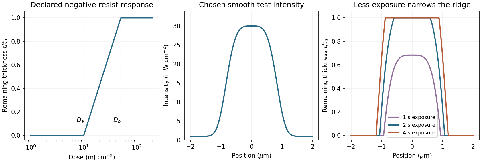
A negative photoresist is removed at low dose and retained at high dose. Its remaining-thickness curve rises from zero above a gel or retention threshold and approaches one above a larger full-retention threshold. A useful schematic model isThe developed profile is $t(x)/t_0=f_{-}[\tau I(x)]$. A central intensity maximum therefore leaves a central ridge, with cleared regions towards the darker sides. Halving exposure narrows and can lower the retained ridge; doubling it broadens the ridge and can raise its shoulders. A saturated central plateau cannot become thicker than the original film in this simple model. If the half-dose peak is below $D_a$, no ridge survives; if it lies between $D_a$ and $D_b$, the centre survives only partially.

The negative-resist thresholds are not supplied, so there is no unique numerical profile or linewidth. The original schematic below declares its own illustrative thresholds and intensity function; it explains the dose mapping without treating a positive-resist curve as measured negative-resist data.

A fully clear opening requires the higher clearing threshold, not merely the onset of thinning. At $\tau =20\mathrm{s}$,The intensity curve crosses this level at about $x=0.25$ and $3.75\mu \mathrm{m}$. Therefore the clear opening is approximatelyThe longer exposure widens the opening because even the relatively dim image tails now accumulate enough exposure dose to clear the positive photoresist. The edge readings are approximate; interpolating a plotted curve does not support nanometre precision.

Use exposure dose $D(x)=I(x)\tau$, with $\mathrm{mW}\times \mathrm{s}=\mathrm{mJ}$. At approximately $x=1.0$ and $3.0\mu \mathrm{m}$, the positive resist just starts to thin. The intensity there is about $5\mathrm{mW}\mathrm{c}{\mathrm{m}}^{-2}$, soAs a consistency check, the fully cleared region begins at approximately $x=1.5$ and ends at $2.5\mu \mathrm{m}$, where the intensity is about $25\mathrm{mW}\mathrm{c}{\mathrm{m}}^{-2}$. Multiplying by $2\mathrm{s}$ gives the clearing dose $50\mathrm{mJ}\mathrm{c}{\mathrm{m}}^{-2}$ at both edges.

Read the straight-line extrapolation on the logarithmic dose axis, rather than the rounded shoulder of the measured curve. The retention and clearing intercepts are approximately $D_0=10$ and $D_{100}=50\mathrm{mJ}\mathrm{c}{\mathrm{m}}^{-2}$. Thus the photoresist contrast isHere the subscripts denote the two dose thresholds used in the supplied definition. The physical positive-resist curve decreases with exposure; $D_{100}$ is the higher clearing dose in that definition, not a statement that the film retains its full thickness there. Graphical intercepts justify roughly two significant figures.

A surface slope converts some vertical displacement into lateral motion of the tip and changes the normal contact geometry. Roughness also changes friction, contact area and local contact stiffness, and can mix cantilever bending, buckling and torsion. A lateral image that follows a height gradient can therefore appear even when the relevant in-plane polarization component is absent.

Record topography and both piezoresponse force microscopy channels simultaneously, and compare the lateral signal with the local slope rather than height alone. Reverse the scan direction to identify frictional contributions, rotate the sample relative to the cantilever, and compare the vector transformation expected for an in-plane response with the geometrical cross-talk. Repeat on a smoother region or a polished specimen, at controlled force and drive amplitude. Track contact resonance or compare sufficiently far from it so that local stiffness does not masquerade as a change in response.

A useful control is a nonpiezoelectric surface of similar roughness. Electrically switching a domain while leaving its topography unchanged provides a further comparison when feasible. No single trace–retrace test proves the absence of cross-talk: genuine in-plane response and slope-induced signals can both transform under rotation, so several controls must agree.

Measure cantilever torsion with the lateral channel of a four-quadrant optical detector. An in-plane surface displacement perpendicular to the cantilever axis twists the cantilever. The reflected laser spot moves sideways, so the left-minus-right detector signal, demodulated at $\omega$ by a lock-in amplifier, gives the amplitude and phase of the lateral piezoresponse. The top-minus-bottom signal primarily records bending.

Displacement along the cantilever axis can instead cause buckling and leak into the nominally vertical channel. Rotate the specimen by $90^{\circ }$ and repeat the measurement to sample the other in-plane component; use a reference specimen and sensitivity calibration before converting a voltage into displacement or force. A torsional spring constant and lever-arm calibration are additionally needed for an actual lateral-force value. Thus lateral piezoresponse is not automatically a calibrated force measurement.

In piezoresponse force microscopy, a conducting atomic force microscopy tip contacts a sample with a counter-electrode. Apply $V(t)=V_{\mathrm{dc}}+V_{\mathrm{ac}}\cos \omega t$. The converse piezoelectric effect produces an oscillatory displacement, approximately $u_{\omega }=d_{\mathrm{eff}}{V}_{\mathrm{ac}}$. Contact with the moving surface bends the cantilever, and a lock-in amplifier records the displacement amplitude and phase relative to the drive.

For opposite out-of-plane ferroelectric domains, the effective piezoelectric coefficient changes sign. Their vertical response therefore differs by approximately $180^{\circ }$ in phase. Equivalent antiparallel domains can have similar amplitudes, while cancellation or reduced response near a wall can produce an amplitude minimum. Phase identifies the relative response sign; an uncalibrated detector phase is not an absolute polarization direction.

Use a small drive below the switching threshold while imaging, a stable contact force and a well-characterized contact resonance. Electrostatic forces, contact stiffness and surface charging can also create signals at the drive frequency; observing contrast alone is insufficient evidence for polarization switching.^[ref]

Diffraction contrast arises because elastic scattering transfers transmitted electron intensity between the direct beam and Bragg diffraction beams. A local change in crystal orientation, strain or thickness changes that transfer. An objective aperture selecting the direct beam makes strongly diffracting regions relatively dark in bright-field transmission electron microscopy; selecting a diffracted beam reverses the selection in dark-field transmission electron microscopy. This is a change in scattering conditions, not necessarily a change in chemical composition.

Three characteristic effects are bend contours, thickness fringes and dislocation contrast. Bend contours follow positions where a gently curved crystal meets a particular Bragg diffraction condition. Thickness fringes arise from thickness-dependent exchange of intensity between coupled transmitted and diffracted waves. A dislocation distorts nearby planes, changing their diffraction condition and producing localized contrast; changing the diffraction vector can suppress particular dislocations. Moiré fringes from overlapping lattices provide another acceptable example, but their coarse spacing is a beat spacing rather than an atomic spacing.

One explanation is block-copolymer kinetic trapping. A solvent-swollen transient sheet structure can be immobilized when a block vitrifies during drying; accurately measured block fractions do not guarantee thermodynamic equilibrium. Thermal annealing above the relevant glass transition, or a controlled nonselective solvent-vapour anneal followed by structural characterization, can test whether the sheets relax toward the bulk composition-appropriate morphology.

A second is surface or confinement selection of lamellar microphase. The diagram describes a bulk reference model. A thin film, preferential wetting at the substrate/free surface or a commensurate confining thickness adds interfacial and geometrical free energy terms that can favour layered arrangements even at an asymmetric global fraction. Unequal layer thicknesses can accommodate $f_A=0.15$; equal block fractions are not required for every layered metastable or confined structure. Varying film thickness and surface chemistry, and comparing bulk-like and confined samples after adequate annealing, distinguishes this explanation from kinetic arrest. Strong conformational asymmetry is another possible departure from the reference model, but an incorrect measured composition need not be invoked.

The Flory interaction parameter ${\chi }_{AB}$ measures the effective free energy penalty for unlike A–B contacts relative to like contacts, and $N$ is the total number of statistical segments per chain. Their product is the segregation strength: contact-energy preference competes with the conformational entropy cost of separating covalently joined blocks. $N$ does not grow during solvent evaporation. For an approximately nonselective solvent, increasing polymer concentration instead increases the effective importance of A–B contacts, so a roughly fixed-composition path moves from weak toward stronger effective segregation.

The diagram's labels are DIS: disordered; S: block-copolymer sphere phase; H: hexagonal cylinder block-copolymer phase; G: double gyroid; L: lamellar microphase. At $f_A=0.15$, A is the minority component and B forms the continuous matrix. Reading the supplied diagram vertically at this composition gives disorder initially, a sphere region when segregation first becomes sufficient, and a cylinder region if sufficiently strong segregation is reached within the displayed range. The thin gyroid and central lamellar regions are not the thermodynamic equilibrium path at this composition. The dry endpoint cannot be fixed numerically without the final ${\chi }_{AB}N$ value. The cited theoretical calculation determines thermodynamic equilibrium phase stability, not a universal evaporation trajectory.^[ref]

Crucially, at least one block is glassy at room temperature. Solvent can initially plasticize it, but solvent loss can raise its effective glass-transition temperature above the processing temperature. Chain relaxation then becomes too slow to equilibrate. Even slow evaporation can therefore freeze disorder, spheres, cylinders or another transient morphology before the thermodynamic equilibrium dry state is reached. Solvent concentration, annealing time and segmental mobility must be followed alongside the phase diagram.

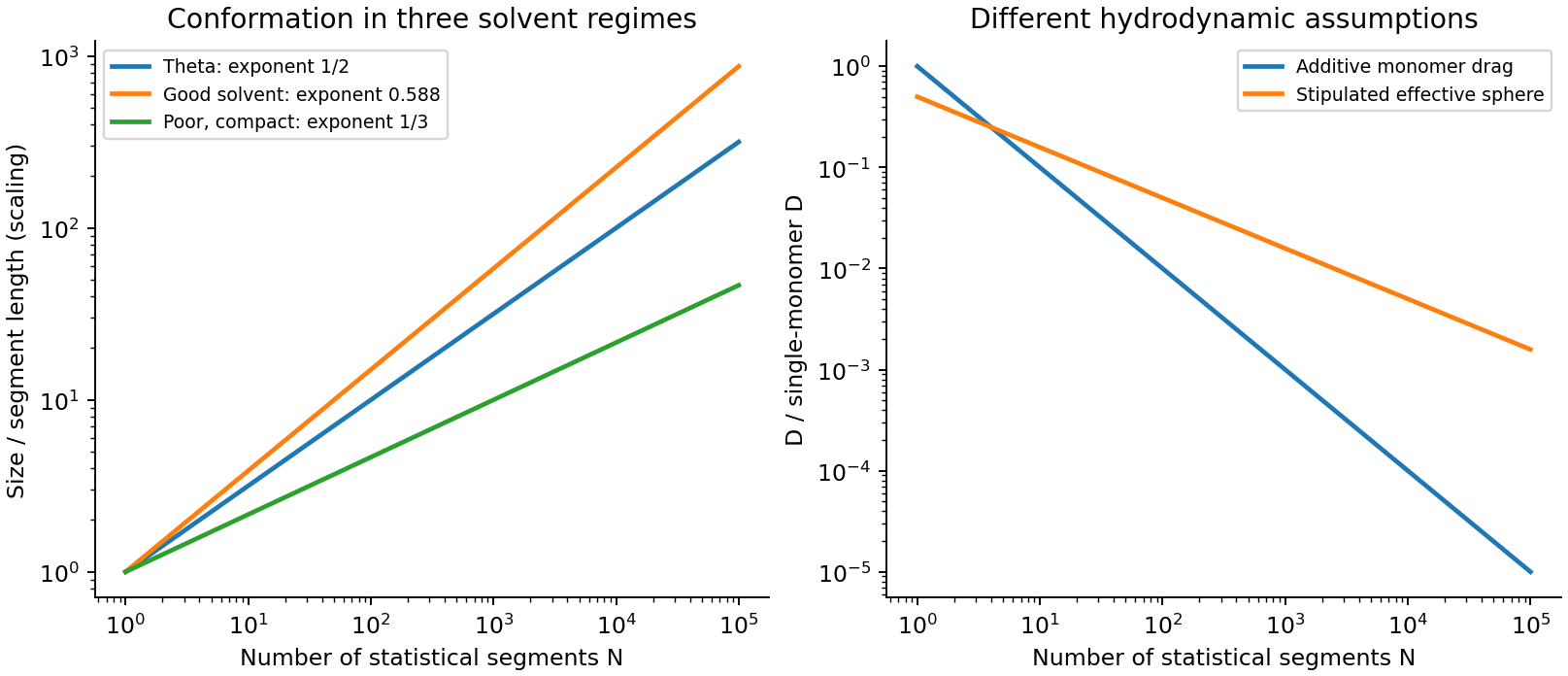
For the stipulated effective-sphere polymer drag, the radius is the end-to-end RMS distance, $R=2a\sqrt{N}$, rather than the single-monomer radius. Its Stokes law and translational diffusion coefficient areUnder the same three-dimensional RMS convention as used above,Thus for sufficiently long chains ($N>4$), this model gives a larger displacement than independent monomer drag: solvent motion couples the parts of a coil, reducing its effective friction relative to $N$ isolated moving beads. The $D\propto N^{-1/2}$ theta-solvent scaling is consistent with the dilute-coil hydrodynamic scaling underlying the Zimm model, but treating a permeable fluctuating coil as a solid sphere with radius exactly $R_{\mathrm{rms}}$ gives only an order-one hydrodynamic approximation. The hydrodynamic radius and end-to-end radius are not generally equal. Neither model by itself restores the long-time constraints of a truly entangled solution.

If the one-dimensional contour statistic in part (iii) is used literally, the comparison of this three-dimensional $d_2$ with that contour RMS is $\sqrt{3/2}{N}^{1/4}$; it compares different coordinates. Using mean radial displacements in both three-dimensional models instead changes both prefactors equally and leaves their ratio unchanged.

At the theta condition, effective excluded volume approximately cancel and a freely jointed ideal chain has $⟨R^2⟩=N{b}^2$. With the stipulated segment length $b=2a$,In a good solvent repulsive excluded volume swells the coil, giving $R\sim b{N}^{\nu }$ with $\nu \simeq 0.588$ in three dimensions, or the Flory approximation $\nu =3/5$. In a poor solvent effective segment attraction favours a compact globule, whose linear size scales as $b{N}^{1/3}$ at roughly fixed internal density. The latter are scaling laws with model-dependent prefactors. A real chemical monomer need not be a statistical Kuhn length; using $2a$ as the independent segment length is part of this question's idealized model.

In the imposed free-draining polymer friction model, the drag coefficients of the $N$ monomers add, giving ${\zeta }_1=N(6\pi \eta a)$ and $D_1=k_{B}T/(6\pi \eta aN)$. Taking the same three-dimensional centre-of-mass RMS convention as part (ii),The polymer is a one-dimensional connected contour, but that alone does not restrict its centre of mass to one spatial axis. If the intended coordinate is instead literal one-dimensional curvilinear motion along an entanglement tube, its RMS contour displacement is $\sqrt{2D_{1}t}=\sqrt{k_{B}Tt/(3\pi \eta aN)}$. That is a different coordinate and should not be compared with a three-dimensional displacement without stating the conversion/model.

Additive local drag is the free-draining Rouse model approximation. It neglects long-range solvent-mediated hydrodynamic interactions and is not a complete theory of an entangled chain. In a tube/reptation description, curvilinear diffusion can scale as $N^{-1}$ while long-time spatial centre-of-mass diffusion scales as $N^{-2}$ after the chain renews its tube. Conversely a dilute unentangled coil can exhibit Zimm model hydrodynamic coupling. Monomer motion, centre-of-mass motion and contour sliding therefore cannot all be identified with the same displacement law.