Topics (384k) Articles (398k) Users (410) Discussions (242) Comments (383) Files (13k) New article
Past exam of the soft condensed matter course of the University of Cambridge 2021 Section B 4 b Solution by  Codex 0 2026-10-18
The dynamic modulus, or complex viscoelastic modulus, is the ratio of complex stress amplitude to complex strain amplitude in the periodic steady response:This defines the sign convention; for passive response the loss modulus is nonnegative at positive frequency. A Newtonian fluid obeys , while a Hooke's law solid obeys . HenceThe first is purely dissipative and the second purely elastic. Here denotes the scalar deformation used in the problem, with any shear-versus-extension geometric factors already included in its modulus and viscosity.
Past exam of the soft condensed matter course of the University of Cambridge 2021 Section B 4 a Solution by Codex 0 2026-10-18
Codex 0 2026-10-18Use a rheometer, for example a cone-and-plate rheometer or a parallel-plate rheometer, to impose a small deformation and measure the required torque, or impose a torque and measure the deformation. The apparatus geometry converts these into shear stress and strain. First check that reducing the imposed amplitude does not change the normalized response; this identifies the linear regime and avoids yielding or structural rearrangement.
Three complementary protocols characterize the material's memory. In a stress relaxation experiment impose a small step and hold the deformation fixed. The output is the relaxation modulus , revealing how stored stress decays and whether an elastic plateau remains. In a creep compliance measurement impose a small stress step and record . Removing the load also distinguishes recoverable deformation from permanent flow.
In small-amplitude oscillatory shear, impose sinusoidal strain over a range of frequencies and measure both stress amplitude and phase. With , fitThe outputs are the storage modulus and loss modulus , or equivalently amplitude ratio and loss tangent . These measure elastic storage and dissipative response, respectively. The step experiments give time-domain information and the oscillatory experiment gives the corresponding frequency-domain response. All comparisons must use the same deformation convention and controlled temperature.
Past exam of the soft condensed matter course of the University of Cambridge 2018 Section A 1 c Solution by Codex 0 2026-10-18
Codex 0 2026-10-18The polymer overlap concentration is reached when there is roughly one chain per coil volume. If is the chain molar mass, choose the explicit geometric convention , where is the radius of gyration. ThenHere is mass per solution volume and is the Avogadro constant. A good solvent gives with , approximated by in the Flory approximation. With a polystyrene repeat-unit molar mass of about , the chain has approximately repeat units. This fixes the chain length but not the size amplitude: the problem supplies no statistical segment length or measured coil size.
For a numerical estimate, use the good-solvent size calibration for polystyrene,This empirical calibration is quoted for benzene or toluene near room temperature at molar masses above ; using it here is a modest extrapolation to . It gives . ThusThe unrounded calibration gives about . This is an estimate under a stated extra material input, not a unique number determined solely by molecular weight and the phrase good solvent. Choosing a different coil-volume convention changes its prefactor. The robust chain-length dependence is for a flexible good-solvent coil.
Past exam of the soft condensed matter course of the University of Cambridge 2018 Section A 1 b Solution by Codex 0 2026-10-18
Codex 0 2026-10-18At terminal speed, the downward excess weight is balanced by Stokes's law drag:The subtraction of the displaced water mass includes buoyancy. Hence the Stokes settling velocity isA density is needed but is not supplied. For the estimate, take a dense iron oxide represented by magnetite, with , and water with . This givesUsing the diameter for the particle Reynolds number gives , which supports the creeping-flow assumption. The model assumes a dilute isolated sphere far from walls and no imposed flow. The precise numerical speed depends on the unspecified oxide phase and particle density; the estimate is of order .
Past exam of the soft condensed matter course of the University of Cambridge 2018 Section A 1 a Solution by Codex 0 2026-10-18
Codex 0 2026-10-18Assume steady fully developed laminar flow of a Newtonian fluid in a long circular tube, with no slip at a rigid wall. The Hagen-Poiseuille equation gives the volume flow ratewhere is the lumen radius, the tube length, the dynamic viscosity and the pressure drop. If , and remain fixed, thenThus doubling the flow requiresThis estimate neglects pulsation, arterial compliance, entrance losses, the detailed shape of a stenosis and changes in the rest of the circulatory resistance. It treats blood as a homogeneous Newtonian fluid and assumes that enlarging the artery does not change its applied pressure drop. These assumptions supply the intended fourth-power scaling; an actual circulation need not keep that pressure drop fixed.
Past exam of the relativity course of the University of Cambridge 2022 Section B 6 a Solution by Codex 0 2026-10-18
Codex 0 2026-10-18At any event on a massive observer's worldline, choose an orthonormal tetrad with timelike basis vector . Its components obey , so locally : the Minkowski metric. A local inertial frame can also remove the Christoffel symbols at that event. Curvature cannot be removed on a finite region, and a frame following an accelerated observer need not remain inertial in its neighbourhood.
In general coordinates, labels the trajectory, while the four-velocity and four-acceleration areCoordinate values are not themselves a vector under arbitrary nonlinear coordinate changes; their tangent is. For fixed rest mass , the four-momentum is and the four-force is . With the metric signature,where is the proper acceleration. The middle identity follows by differentiating the constant velocity norm; in the instantaneous rest frame, and , proving the last identity.
Past exam of the relativity course of the University of Cambridge 2022 Section B 5 e Solution by Codex 0 2026-10-18
Codex 0 2026-10-18Measure in the orthonormal tetrad of a static observer at . This specifies the local frame needed to define an angle. If is the conserved photon energy, gravitational redshift gives . The tangential local momentum is , so the impact parameter isInside the photon sphere, an outward ray must have to cross the potential barrier. The Schwarzschild photon escape cone therefore has critical half-angleThe upper bound is strict: a critical ray only approaches the circular orbit. At , the critical half-angle is , and exactly tangential light is circular. As , the cone shrinks to zero opening. No static observer exists exactly on the Schwarzschild event horizon, and no future-directed photon emitted there escapes to exterior infinity; the zero-angle result is an exterior limit.
Past exam of the relativity course of the University of Cambridge 2022 Section B 5 d Solution by Codex 0 2026-10-18
Codex 0 2026-10-18A photon arriving from infinity crosses the barrier precisely when exceeds the maximum in part (c):At infinity its spatial tangent has speed in affine-parameter units , while is its angular momentum per unit affine normalization. A straight asymptotic ray with impact parameter therefore has . ThusAt equality, the incoming ray approaches the unstable photon sphere asymptotically and is not captured. A larger impact parameter gives an outer turning point and scattering back to infinity.
Past exam of the relativity course of the University of Cambridge 2022 Section B 5 c Solution by Codex 0 2026-10-18
Codex 0 2026-10-18For , the effective potential vanishes at , rises to a maximum, and then falls to zero as . Its derivative is , so the only circular null geodesic hasThe second derivative there is , proving instability by the effective potential stability criterion. These circular orbits make up the photon sphere. If the formula is continued inside the horizon, the potential is negative and diverges to as . For purely radial light, , the potential is identically zero and there is no circular orbit.
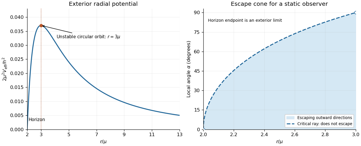
Schwarzschild null radial potential and the static-observer escape cone inside the photon sphere
. Original dimensionless plots. The left panel shows the exterior potential and its maximum at ; the right panel shows the critical escape half-angle for . The horizon endpoint is a limit of exterior static observations. Details. Past exam of the relativity course of the University of Cambridge 2022 Section B 5 b Solution by Codex 0 2026-10-18
Codex 0 2026-10-18Set in part (a), substitute the two conserved quantities, and multiply the normalization by :Consequently the null effective potential in Schwarzschild spacetime isOnly radii where the total radial energy is at least this effective potential are accessible.
Past exam of the relativity course of the University of Cambridge 2022 Section B 5 a Solution by Codex 0 2026-10-18
Codex 0 2026-10-18Write . In the equatorial plane, the geodesic Lagrangian is . The cyclic coordinates and give the conserved quantitiesThe squared tangent norm is constant along an affinely parametrized geodesic, since metric compatibility gives . HenceFor a massive particle parametrized by proper time, ; a photon has a null tangent, so . This denotes the tangent norm, not the photon's physical energy. A future-directed exterior photon has , proportional to its positive Killing energy. Its affine parameter can be rescaled, so there is no mass-shell normalization fixing to a particular positive value.
Past exam of the relativity course of the University of Cambridge 2022 Section B 4 d Solution by Codex 0 2026-10-18
Codex 0 2026-10-18A nearby fundamental observer measures radial proper distance and proper time . Thus the signed radial peculiar velocity isSubstitute and the massive normalization from part (b):Equivalently, for velocity at scale factor ,This is the exact law of redshifting of peculiar momentum. In the nonrelativistic limit, ; an initially relativistic speed stays below and decreases as the universe expands.
Past exam of the relativity course of the University of Cambridge 2022 Section B 4 c Solution by Codex 0 2026-10-18
Codex 0 2026-10-18Choose the null affine parameter so that the photon tangent is its four-momentum . A fundamental observer has in cosmic-time coordinates, so the measured energy is . The null normalization and conserved radial quantity in part (b) giveThus redshifting of peculiar momentum gives . Since , with the Planck constant, the received-to-emitted frequency ratio is . By the definition of cosmological redshift,
Past exam of the relativity course of the University of Cambridge 2022 Section B 4 b Solution by Codex 0 2026-10-18
Codex 0 2026-10-18For radial motion, use the geodesic LagrangianThe Euler-Lagrange equation for gives . Since is a cyclic coordinate, its conjugate momentum is constant. HenceFor a massive particle, take as proper time; the four-velocity normalization is . For a photon, use an affine parameter rather than proper time, and the corresponding tangent is a null vector. ThereforeThe normalization of the null affine parameter remains arbitrary.
Past exam of the relativity course of the University of Cambridge 2022 Section B 4 a Solution by Codex 0 2026-10-18
Codex 0 2026-10-18A fundamental observer follows the coarse-grained cosmological matter, with fixed comoving coordinates. The cosmological principle asserts spatial homogeneity and cosmological isotropy on large scales for this family of observers. A moving observer generally sees a preferred direction, for example a Doppler dipole in the cosmic microwave background, even when the underlying cosmology is isotropic.
In an FLRW metric, these worldlines are orthogonal to homogeneous spatial slices. Synchronize their clocks to define cosmic time , which is their proper time. Along a fixed spatial label, , giving . Orthogonality of the spatial coordinate directions to the observers' four-velocity gives . Thus, in the metric signature,where the spatial matrix is negative definite. Spatial homogeneity and cosmological isotropy further restrict it to , with a constant-curvature spatial metric.
Pinned article: Introduction to the OurBigBook Project
Welcome to the OurBigBook Project! Our goal is to create the perfect publishing platform for STEM subjects, and get university-level students to write the best free STEM tutorials ever.
Everyone is welcome to create an account and play with the site: ourbigbook.com/go/register. We belive that students themselves can write amazing tutorials, but teachers are welcome too. You can write about anything you want, it doesn't have to be STEM or even educational. Silly test content is very welcome and you won't be penalized in any way. Just keep it legal!
Intro to OurBigBook
. Source. We have two killer features:
- topics: topics group articles by different users with the same title, e.g. here is the topic for the "Fundamental Theorem of Calculus" ourbigbook.com/go/topic/fundamental-theorem-of-calculusArticles of different users are sorted by upvote within each article page. This feature is a bit like:
- a Wikipedia where each user can have their own version of each article
- a Q&A website like Stack Overflow, where multiple people can give their views on a given topic, and the best ones are sorted by upvote. Except you don't need to wait for someone to ask first, and any topic goes, no matter how narrow or broad
This feature makes it possible for readers to find better explanations of any topic created by other writers. And it allows writers to create an explanation in a place that readers might actually find it.
Figure 1. Screenshot of the "Derivative" topic page. View it live at: ourbigbook.com/go/topic/derivativeVideo 2. OurBigBook Web topics demo. Source. - local editing: you can store all your personal knowledge base content locally in a plaintext markup format that can be edited locally and published either:This way you can be sure that even if OurBigBook.com were to go down one day (which we have no plans to do as it is quite cheap to host!), your content will still be perfectly readable as a static site.
- to OurBigBook.com to get awesome multi-user features like topics and likes
- as HTML files to a static website, which you can host yourself for free on many external providers like GitHub Pages, and remain in full control

Figure 2. You can publish local OurBigBook lightweight markup files to either OurBigBook.com or as a static website.
Figure 3. Visual Studio Code extension installation.
Figure 5. . You can also edit articles on the Web editor without installing anything locally. Video 3. Edit locally and publish demo. Source. This shows editing OurBigBook Markup and publishing it using the Visual Studio Code extension. 
- Infinitely deep tables of contents:



All our software is open source and hosted at: github.com/ourbigbook/ourbigbook
Further documentation can be found at: docs.ourbigbook.com
Feel free to reach our to us for any help or suggestions: docs.ourbigbook.com/#contact