A physical delay is a time, whereas the stated $\lambda /(4\sqrt{2})$ is a length. First interpret it literally as an additional optical path length $\ell =\lambda /(4\sqrt{2})$ in arm 1, with the other arm unchanged. In vacuum this delays its full field by ${\tau }_d=\ell /c$. The exact stationarity argument from part (b) then givesDelaying arm 2 changes the plus sign before ${\tau }_d$ to a minus sign. As a function of $y$, the arm-1 result is the old pattern evaluated at $y+\ell /\sqrt{2}=y+\lambda /8$.

For a quasi-monochromatic source, ${\tau }_d$ is much shorter than the coherence time. The envelope correlation can then be treated as unchanged, while the carrier wave phase cannot:HenceThis literal optical-path delay is not a quarter-cycle wave phase shift. If the intended length instead specifies a displacement of the entire recorded fringe pattern by one quarter of its period, $\Delta y=\lambda /(4\sqrt{2})$, the equivalent delay is $\sqrt{2}\Delta y/c=\lambda /(4c)$ and the wave phase shift is $\pi /2$. Under that different interpretation the narrow-band result is $I_0+\mathrm{Im}\Gamma (\tau (y))$, with its sign reversed for the opposite displacement. The exact expression is still a shifted argument of $\Gamma$, not merely a wave phase multiplier when the envelope varies. The original wording does not specify such a fringe-pattern displacement, so these interpretations must be distinguished.

The $x$ axis lies along the mean Poynting vector. A two-dimensional optical camera sensor intended to sample many $x$ positions at once would have to lie along the energy flow, where it receives no normal flux in the ideal geometry; a side-view optical camera also sees no light from an empty nonscattering propagation region. Putting a detector normal to $x$ measures one transverse section instead, and absorbs the light before a downstream detector can sample the same rays.

One could translate a detector to successive $x$ positions or introduce a scattering screen, but that is a different measurement. Moreover the ideal result here is already the constant $I(x)=2I_0$, so it contains no longitudinal optical coherence structure for the optical camera to resolve. The difficulty is the longitudinal sampling geometry, rather than a hidden $x$-fringe period.

On the $x$ axis the two geometric delays are identical:Their field wave amplitudes therefore add as equal copies at zero relative delay. Stationarity removes dependence on the common delay, givingindependent of $x$ in the ideal overlapping plane-wave region. The corresponding mean normal energy flux through a transverse plane is $\sqrt{2}{I}_0$. There is no increasing path difference along the bisector, so finite temporal optical coherence does not produce a longitudinal visibility envelope on this axis.

For each beam in vacuum, its magnetic field is ${\mathbf{B}}_j={\hat{\mathbf{k}}}_j\times {\mathbf{E}}_j/c$. Write the two complex scalar contributions, including the beam splitter factor, as $u_1=f(t-t_1)/\sqrt{2}$ and $u_2=f(t-t_2)/\sqrt{2}$. Since their electric fields are both along $z$,The optical-cycle and ensemble-averaged Poynting vector isThe mean individual light intensities are equal, soThus energy flows along the bisector of the two beam directions, crossing a detector plane normal to $x$. Such a sensor can in principle record the variation across its $y$ coordinate. Its actual normal energy flux is $I(y)/\sqrt{2}$ in the normalization used above; this fixed factor does not change interferometric visibility.

There is a practical resolution condition in addition to the direction of energy flow. The interference fringe spacing $\lambda /\sqrt{2}$ is very small, so direct pixels would need spacing no larger than $\lambda /(2\sqrt{2})$ as required by the Nyquist–Shannon sampling theorem, or optical magnification and sufficient angular aperture to preserve both incident directions. An ordinary optical camera with much larger effective pixels averages the interference fringes. The Poynting-vector argument establishes the allowed measurement geometry, not guaranteed resolution with any optical camera.

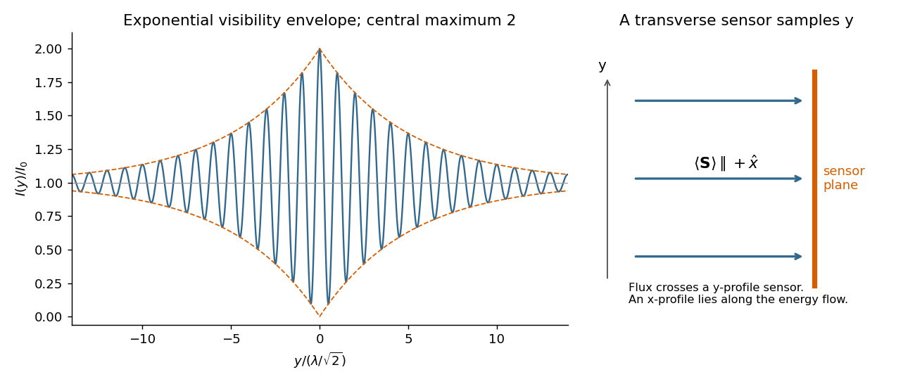
A line with lifetime broadening has a Lorentzian line shape. Write its half-width at half-maximum in angular-frequency units as $\kappa >0$. The Wiener-Khinchin theorem, or the Fourier transform of the Lorentzian, givesTherefore in vacuumThe sketch is a cosine fringe pattern about baseline $I_0$, bounded by $I_0[1\pm e^{-\sqrt{2}\kappa |y|/c}]$. Its central value is $2I_0$, its spatial interference fringe spacing is $\lambda /\sqrt{2}$, and its visibility decays on length $c/(\sqrt{2}\kappa )$. For an isolated transition whose population lifetime is $T_1$ and which has no extra dephasing, $\kappa =1/(2T_1)$, so the field coherence time is $2T_1$, not $T_1$. Introducing $\kappa$ avoids confusing population, wave amplitude and spectral-width conventions when no numerical linewidth is given.

The given spatial and carrier factors combine into retarded copies of the same random field:On the $y$ axis, $t_1=ky/(\sqrt{2}\omega )$ and $t_2=-ky/(\sqrt{2}\omega )$. Expand the squared electric-field wave amplitude. Each self term contributes $I_0/2$, and the two cross terms together contribute the real part of the full-field correlation. Stationarity and $\Gamma (-\tau )=\Gamma (\tau {)}^{\ast }$ giveIn vacuum, $k=\omega /c$ and $\tau (y)=\sqrt{2}y/c$. Reversing the delay convention replaces $\tau$ by $-\tau$ without changing this real-part result. This $I$ is the electric-field light intensity convention of the question. For two nonparallel waves it should not automatically be identified with the magnitude of the net Poynting vector; part (d) gives that geometric conversion explicitly.

Take $f(t)=a(t)e^{-i\omega t}$ at a fixed reference point, and define the full-field temporal optical coherence function byThe angle brackets denote an ensemble expected value, or a sufficiently long time average when justified. The factor $C$ puts $\Gamma$ in light intensity units for the chosen peak complex-field convention. The normalized first-order optical coherence is $g^{(1)}(\tau )=\Gamma (\tau )/\Gamma (0)$ for a stationary source.

“Independent of absolute time” means the second moment depends on the time difference $\tau$ but not on the starting time $t$: shifting both observation times by the same amount leaves it unchanged. Together with a constant mean this is second-order or weak stationarity; it does not mean that the random electric field is constant in time. Put $I_0=\Gamma (0)=C⟨|a{|}^2⟩$. The full-field convention is important: an envelope-only correlation omits $e^{-i\omega \tau }$ and must have that carrier factor restored before deriving optical interference fringes.

The circular eigenmode orthogonal projection matrices obey $P_{\pm }^2=P_{\pm }$, $P_{+}{P}_{-}=0$ and $P_{+}+P_{-}=I$. Define the uniform-medium generatorExpanding its matrix exponential by its power series and using these projection identities givesEquivalently, with $Q=\left(\begin{array}{cc}0& i\\ -i& 0\end{array}\right)$, one has $Q^2=I$, $K=\gamma I+\delta Q$ and $e^{-Kz}=e^{-\gamma z}[I\cosh (\delta z)-Q\sinh (\delta z)]$. This is exactly the corrected matrix of part (d). The entries of $K$ have units of inverse length, and the map satisfies $d\mathcal{J}/dz=-K\mathcal{J}$, $\mathcal{J}(0)=I$ and the homogeneous propagation law $\mathcal{J}(z_1+z_2)=\mathcal{J}(z_1)\mathcal{J}(z_2)$.

The extra ${\mathrm{sech}}^2$ factor in the printed version violates this last law for nonzero $\delta$, so it cannot be generated by one constant $K$ with the stipulated eigenvalues. The constant-$K$ description assumes uniform coefficients and fixed circular eigenmodes.

Write ${\gamma }^{\pm }=-i{\beta }^{\pm }$, $\overline{\beta }=({\beta }^{+}+{\beta }^{-})/2$ and $\chi =({\beta }^{+}-{\beta }^{-})z/2$. Then $\gamma z=-i\overline{\beta }z$ and $\delta z=-i\chi$. With $\cosh (-i\chi )=\cos \chi$ and $\sinh (-i\chi )=-i\sin \chi$, the corrected matrix becomesThe scalar is a common propagation wave phase and the real rotation matrix rotates the input linear polarization through $\chi$. There is no attenuation and no generated ellipticity: the field map is a unitary matrix. The two circular eigenmodes accumulate different wave phases, giving circular birefringence and optical activity.

The correct unfactored matrix remains finite where $\cos \chi =0$. In contrast, the printed $\mathrm{sech}$ form would give $e^{i\overline{\beta }z}{\sec }^2\chi$ times the rotation matrix, including unphysical divergent gain in this stipulated lossless case. This provides a direct physical check on the correction in part (d).

When ${\gamma }^{\pm }={\alpha }^{\pm }$ are real, $\gamma$ and $\delta$ are real. The two opposite circular polarizations retain their wave phases but are attenuated at different wave amplitude rates. This circular dichroism changes the ellipticity without rotating the principal axis of the ellipse.

For input $E_0\hat{\mathbf{x}}$, the corrected Jones matrix givesThe common factor $e^{-\gamma z}$ describes the mea wave amplitude attenuation. The $\cosh (\delta z)$ factor reflects the sum of the two transmitted modal wave amplitudes; $\tanh (\delta z)$ fixes their imbalance and hence the signed ellipticity. The real field has components proportional to $\cosh (\delta z)\cos \omega t$ and $\sinh (\delta z)\sin \omega t$, soThe ellipse's principal axis stays along the original input direction. For large differential optical depth it approaches the less attenuated circular eigenmode. A passive medium has ${\alpha }^{\pm }\ge 0$, or $\gamma \ge |\delta |$, so the growing hyperbolic function factor does not imply net optical gain. Using the printed $\mathrm{sech}$ prefactor would give a spurious extra attenuation inconsistent with the modal laws.

There are errors in the original PDF at this point, not merely in the TeX transcription. The second exponential must denote the eigenvalue ${\lambda }_{-}(z)=e^{-{\gamma }^{-}z}$, not the propagation coefficient itself. More substantially, the printed prefactor $\mathrm{sech}(\delta z)$ is inconsistent with the stated exponential eigenvalues. It must be $\cosh (\delta z)$. The original's primed Jones-matrix label distinguishes the distributed component from the earlier static matrix; below write $\mathcal{J}(z)$ to avoid confusing that prime with a derivative.

Complex eigenvalues have no intrinsic largest/smallest ordering, so $+$ and $-$ are modal labels. Keep the circular eigenvectors fixed, put $\gamma =({\gamma }^{+}+{\gamma }^{-})/2$ and $\delta =({\gamma }^{+}-{\gamma }^{-})/2$, and use the spectral decomposition from part (c):Its diagonal entries are $(e^{-{\gamma }^{+}z}+e^{-{\gamma }^{-}z})/2=e^{-\gamma z}\cosh (\delta z)$, and its upper off-diagonal entry is $i(e^{-{\gamma }^{+}z}-e^{-{\gamma }^{-}z})/2=-i{e}^{-\gamma z}\sinh (\delta z)$. ThereforeWhere $\cosh (\delta z)\ne 0$, this can be factored asThe unfactored expression is valid even at zeros of the cosine-like factor when $\delta$ is imaginary. The printed expression is ${\mathrm{sech}}^2(\delta z)$ times this correct matrix; its eigenvalues are consequently $e^{-{\gamma }^{\pm }z}{\mathrm{sech}}^2(\delta z)$ rather than those specified. A second check is $\det \mathcal{J}=e^{-2\gamma z}$, whereas the printed version has determinant $e^{-2\gamma z}{\mathrm{sech}}^4(\delta z)$. Thus the requested printed identity cannot be proved except in the degenerate case $\delta =0$; the following parts use the consistent propagator.

The normalized circular eigenvectors from part (a) define the orthogonal projection matricesThus the spectral decomposition of the Jones matrix isThis simply substitutes $a=({\lambda }_{+}+{\lambda }_{-})/2$ and $b=({\lambda }_{+}-{\lambda }_{-})/2$ and makes each eigenmode's wave amplitude transmission explicit.

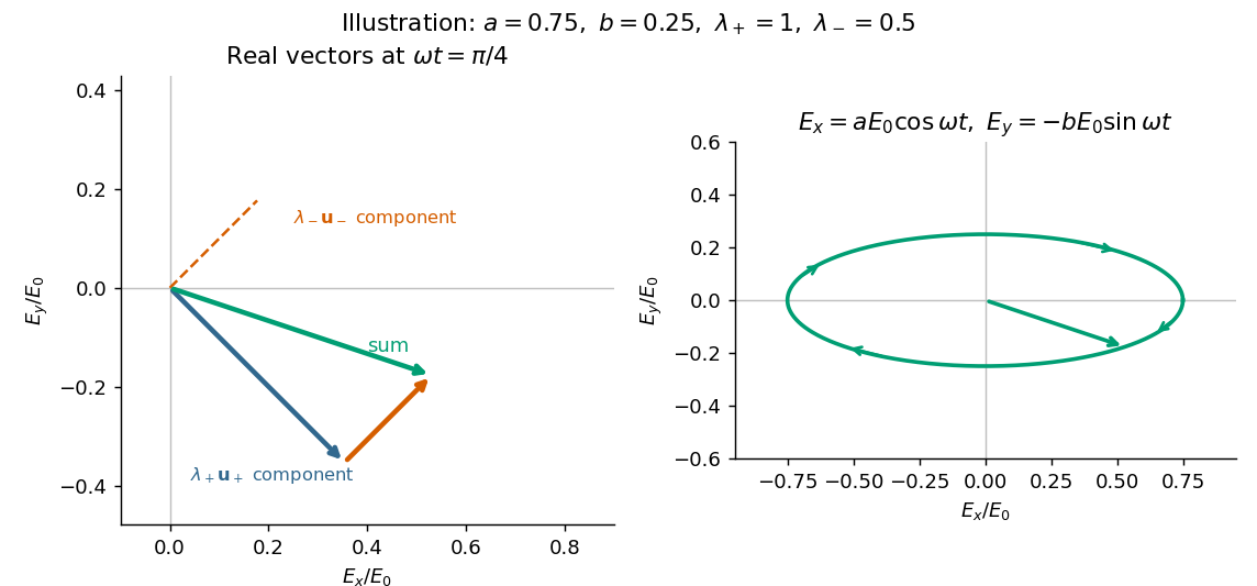
Take an incident field along $\hat{\mathbf{x}}$, without loss of generality because this component has the same circular eigenmodes for every direction of input linear polarization. Resolve its Jones vector into equal circular components:Using the complex amplitude convention $\mathrm{Re}[\mathbf{E}{e}^{-i\omega t}]$, the real circular contributions areThey counter-rotate and add toIn general the tip traces an ellipse with semiaxis lengths $|a|E_0$ and $|b|E_0$. Equal transmitted circular wave amplitudes produce a line; removal of one circular mode, ${\lambda }_{+}=0$ or ${\lambda }_{-}=0$, produces a circle. The special zero-output case has no defined polarization of waves.

The characteristic polynomial of the given Jones matrix isso a convenient choice of eigenvalue labels isDirect multiplication gives $J{\mathbf{u}}_{\pm }={\lambda }_{\pm }{\mathbf{u}}_{\pm }$, and ${\mathbf{u}}_{+}^{†}{\mathbf{u}}_{-}=0$. They represent opposite circular polarizations. Since $a,b$ are real, $J$ is a Hermitian matrix and both eigenvalues are real, but they need not be positive. A negative eigenvalue adds a wave phase reversal to that mode. The labels are algebraic: ${\lambda }_{+}$ is the larger numerical eigenvalue only when $b\ge 0$. If $b=0$, the eigenvalue is degenerate and every nonzero Jones vector is an eigenvector; the circular pair remains a valid basis.

Distinguish reflection at the input terminal, reflection at the receiving load, and a returned signal that traverses the free-space link twice. The input antenna is initially matched, so its direct terminal reflection is zero.

In the usual weak-coupling, matched-port two-port network model for the antenna pair, let the forward and reverse wave amplitude transfer coefficients be $t_{21}$ and $t_{12}$. Electromagnetic reciprocity gives equal power transfer factors $|t_{21}{|}^2=|t_{12}{|}^2=\mathcal{F}$, where $\mathcal{F}=(G_a\lambda /(4\pi d){)}^2$ from part (a). The receiving-load reflection returns wave amplitude $t_{12}{\Gamma }_L{t}_{21}$ to the original input port. The load-mismatch contribution to the returned power is thereforeFor fixed gains and impedances this returned power scales as ${\lambda }^4$: it contains two link traversals. By contrast, the reflected power at the receiving load before that return traversal is $P_i\mathcal{F}|{\Gamma }_L{|}^2\propto {\lambda }^2$. Calling that local reflected power the power already back in the input line would omit one propagation loss.

The original wording does not specify an antenna scattering model. The boxed result is the load-dependent echo in an ideal matched-port link, with structural scattering and residual input coupling neglected. The actual total input return can include coherent scattering from the receiving antenna even when ${\Gamma }_L=0$; gains and effective areas alone do not specify that background. If “reflected back” means only the direct reflection at the stated matched transmitting antenna, its value is $0$. These meanings should not be conflated; the ${\lambda }^4$ result requires the two-pass echo interpretation and its stated model.

The transmitting antenna is matched to its input transmission line, so its real terminal electrical resistance is $Z_i$. The identical receiving antenna has the same electrical impedance at the operating frequency. Its available received power for a matched load is the incident energy flux times its antenna effective area:The real receiving load is $Z_t$, so its voltage-wave reflection coefficient relative to $Z_i$ is ${\Gamma }_L=(Z_t-Z_i)/(Z_t+Z_i)$. The fraction of available power delivered to the output line isConsequently, neglecting path losses, mismatch of polarization of an electromagnetic wave and line losses,This is the Friis transmission equation with a receiving impedance-mismatch factor. For fixed $P_i,G_a,d,Z_i,Z_t$, it scales as ${\lambda }^2$. That scaling is conditional on holding antenna gain fixed: a fixed physical aperture can instead have $G_a\propto {\lambda }^{-2}$, and any wavelength dependence of the impedances also enters the expression. The matched-output check $Z_t=Z_i$ gives $P_t=P_i\mathcal{F}$.

Now take $\hat{\mathbf{n}}=(0,\sin \psi ,\cos \psi )$, with the same angle to the incident $z$ direction. The perpendicular direction is $\hat{\mathbf{x}}$ and the in-plane transverse direction is $(0,\cos \psi ,-\sin \psi )$. The roles of the two electric dipole populations interchange: $x$ electric dipoles radiate at full strength, whereas the observed wave amplitude from a $y$ electric dipole is reduced by $\cos \psi$.

Thus $I_{\perp }=C{N}_1$ and $I_{\parallel }=C{N}_2{\cos }^2\psi$, givingThis is also obtained by the symmetry $x\leftrightarrow y$, $N_1\leftrightarrow N_2$ in part (a). For $N_1=N_2$, both planes give the familiar Rayleigh scattering degree of polarization ${\sin }^2\psi /(1+{\cos }^2\psi )$: the diffuse signal is unpolarized forward and fully linearly polarized at right angles. At a dark direction with zero denominator, no degree of polarization can be measured.