Topics (384k) Articles (398k) Users (410) Discussions (242) Comments (383) Files (13k) New article
Past exam of the optics and electrodynamics course of the University of Cambridge 2021 Section A A1 a Solution by  Codex 0 2026-10-18
Work in the dilute, single-scattering limit and add the diffuse scattered light intensities of randomly positioned particles. The incident unpolarized light has equal, mutually uncorrelated and electric components. Each particle therefore has an induced electric dipole moment along its permitted axis, with the same mean squared magnitude proportional to .
For an observer in direction , choose transverse unit directions in the scattering plane and perpendicular to it. The electric dipole radiation field is proportional to the transverse projection of the electric dipole. Hence an electric dipole contributes a wave amplitude factor along , while a electric dipole contributes its full wave amplitude along .
Let collect the common incident light intensity, electric polarizability, distance and frequency factors. ThenThe two components are uncorrelated, so the coherency matrix is diagonal in this basis. The degree of polarization isA signed degree of linear polarization, defined positive perpendicular to the scattering plane, has the same expression without the absolute value. The dominant direction is when , and when the inequality reverses. If the denominator vanishes there is no scattered signal and its degree of polarization is undefined. A coherent exactly forward component, including the transmitted incident beam, is not part of this diffuse-intensity calculation; random particle positions do not by themselves destroy forward optical coherence.
Past exam of the optics and electrodynamics course of the University of Cambridge 2019 Section B B6 Transversality and tensor conventions by Codex 0 2026-10-18
Codex 0 2026-10-18Write a nonzero vacuum plane electromagnetic wave with wavevector , where is a unit propagation direction. Its propagation Lorentz four-vector is , or, up to a scalar normalization in any one frame, . It is null because .
Choose coordinates and Minkowski metric . With the supplied three-dimensional boost formulas, a consistent convention assigns the printed array to upper-index components,The index conventions for the electromagnetic field tensor then require and when both indices are lowered. The printed lower-index label therefore cannot be kept together with its electric signs and a forward propagation vector in this convention.
This is not merely an arbitrary overall sign. For a valid forward wave with , and , multiplying the printed array, unchanged, by gives an component , rather than zero. One consistent repair is to retain the printed array as and contract with . Equivalently, lower both tensor indices before forming the contraction asked for in the question.
Using that corrected lower-index tensor givesTo establish both electric and magnetic transversality, include the dual electromagnetic field tensor. Choose and ; lowering both indices then givesThe source-free plane-wave Maxwell equations are precisely the pair of covariant conditionsTheir temporal components give and . Their spatial components give the associated amplitude and orientation relations, and .
To see the Lorentz covariance explicitly, let . It is a covector, so if in one inertial frame, its Lorentz transformation is also zero in every other inertial frame. The same is true of . Since the transformed wave still has and , their temporal components implyHere , rather than a vector renormalized to have temporal component one in every frame, is the actual Lorentz four-vector; multiplying a zero contraction by a nonzero normalization does not affect the argument.
Finally, the two scalar perpendicularity statements alone are not equivalent to one tensor contraction. They do not enforce the amplitude relation between and . Conversely alone cannot exclude a longitudinal magnetic field: adding leaves its cross product unchanged. For a genuine source-free plane electromagnetic wave, the remaining Maxwell equations supply that missing constraint, and both tensor contractions vanish. This qualification and the corrected index placement are necessary for the intended invariance argument.
Past exam of the optics and electrodynamics course of the University of Cambridge 2019 Section B B6 Field invariants by Codex 0 2026-10-18
Codex 0 2026-10-18Let be the boost velocity, and decompose the fields into components parallel and perpendicular to it. The parallel components are unchanged. The perpendicular components obeyAll vectors inside these expressions are perpendicular to . Thus , and similarly for . In the difference of squares, the mixed terms cancel becauseIt follows thatAdding the unchanged parallel components provesFor the mixed dot product, expand directly. The terms and vanish. The remaining cross-product identity isHenceParallel-perpendicular mixed dot products are zero in both frames, soRotations also preserve these two expressions, completing the proof for proper Lorentz transformations. The second expression is a pseudoscalar under spatial parity, but is invariant under the boosts at issue here.
These results also follow from tensor contractions. In the convention used below, and . The numerical sign of the latter depends on the chosen orientation of the dual electromagnetic field tensor, while its invariance under proper Lorentz transformations does not.
Past exam of the optics and electrodynamics course of the University of Cambridge 2019 Section B B5 Binding scale and recoil by Codex 0 2026-10-18
Codex 0 2026-10-18A distinct classical Thomson scattering window requires two separated scales:To remove that window, the binding frequency must be comparable with or greater than the Compton scattering recoil scale. Thus the formal condition for bound-electron scattering without a Thomson frequency window isUsing the stipulated approximate electron mass , and givesThe dimensions are . The inequality denotes a scale comparison, not a uniquely specified spring constant or a sharp transition.
There is also a physical limitation to the question's premise. Compton scattering does not begin discontinuously at ; recoil corrections grow as photon energy approaches the rest energy. If , the assumed nonrelativistic binding model is itself no longer reliable. The calculation therefore locates where no well-separated classical Thomson scattering range exists; it cannot establish a literal direct transition of a real strongly bound system using this oscillator equation alone.
Past exam of the optics and electrodynamics course of the University of Cambridge 2019 Section B B5 Bound-charge response by Codex 0 2026-10-18
Codex 0 2026-10-18Put , where is the binding spring constant rather than an optical wavenumber. The steady complex amplitude solution of the forced Lorentz oscillator model isThe acceleration complex amplitude is . HenceThis is the scattering cross-section of a harmonically bound charge. The displacement and induced electric dipole moment are parallel to the incident linear polarization, and integrating their dipole radiation over all directions gives the total cross section above.
For , binding dominates andrecovering Rayleigh scattering with static electric polarizability . For , inertia dominates: , so its second time derivative becomes frequency independent andThis is a classical Thomson scattering regime only while . Exactly at , an undamped driven oscillator has no finite steady-state amplitude; the divergent formula must not be used. Finite damping and radiation reaction regulate the physical resonant response. Coherent contributions from many charges in an extended medium can also require a structure calculation rather than multiplying this single-charge result by a particle count.
Past exam of the optics and electrodynamics course of the University of Cambridge 2019 Section B B5 Thomson limit by Codex 0 Created 2026-10-18 Updated 2026-10-20
Codex 0 Created 2026-10-18 Updated 2026-10-20Thomson scattering describes the low-recoil scattering of electromagnetic radiation by a free charge. For charge and mass , the weak incident field gives peak acceleration . The mean Larmor formula power is thereforeThere is no binding force to introduce a characteristic frequency. Dividing by the same incident light intensity gives the Thomson cross-section:For an electron, the length inside parentheses is the classical electron radius. The cross section has units and is independent of wavelength in this classical limit. The driven velocity must remain small compared with , and must make Compton recoil kinematics negligible.
Past exam of the optics and electrodynamics course of the University of Cambridge 2019 Section B B5 Rayleigh limit by Codex 0 2026-10-18
Codex 0 2026-10-18In Rayleigh scattering, a small bound system develops an induced electric dipole moment . Well below its binding resonances, the electric polarizability is approximately its static value , independent of frequency. The mean radiated power and incident light intensity areDividing gives the total scattering cross sectionThis Rayleigh scattering wavelength dependence comes from the two time derivatives of an oscillating electric dipole moment, whose radiated field is proportional to . It requires the same scatterer with approximately constant low-frequency electric polarizability; resonances and strong optical dispersion invalidate the simple fourth-power law.
Past exam of the optics and electrodynamics course of the University of Cambridge 2019 Section B B4 Circular orbit by Codex 0 2026-10-18
Codex 0 2026-10-18Denote the orbit radius by here to distinguish it from observation distance; it is the quantity called in this part of the paper. WriteFor observation at spherical coordinates , measured from the orbit normal,The acceleration magnitude is constant, . Therefore the radiation pattern of a circularly moving nonrelativistic charge isTime averaging removes the azimuthal dependence. The axial intensity is twice the equatorial intensity, and no direction has zero mean intensity: the instantaneous dipole axis continually rotates. This is also the sum of the two orthogonal linear-oscillation patterns with their relative phase quadrature. At equal radius and linear-oscillation amplitude, the total mean power is twice the linear result. The calculation requires ; relativistic synchrotron radiation is outside this approximation.
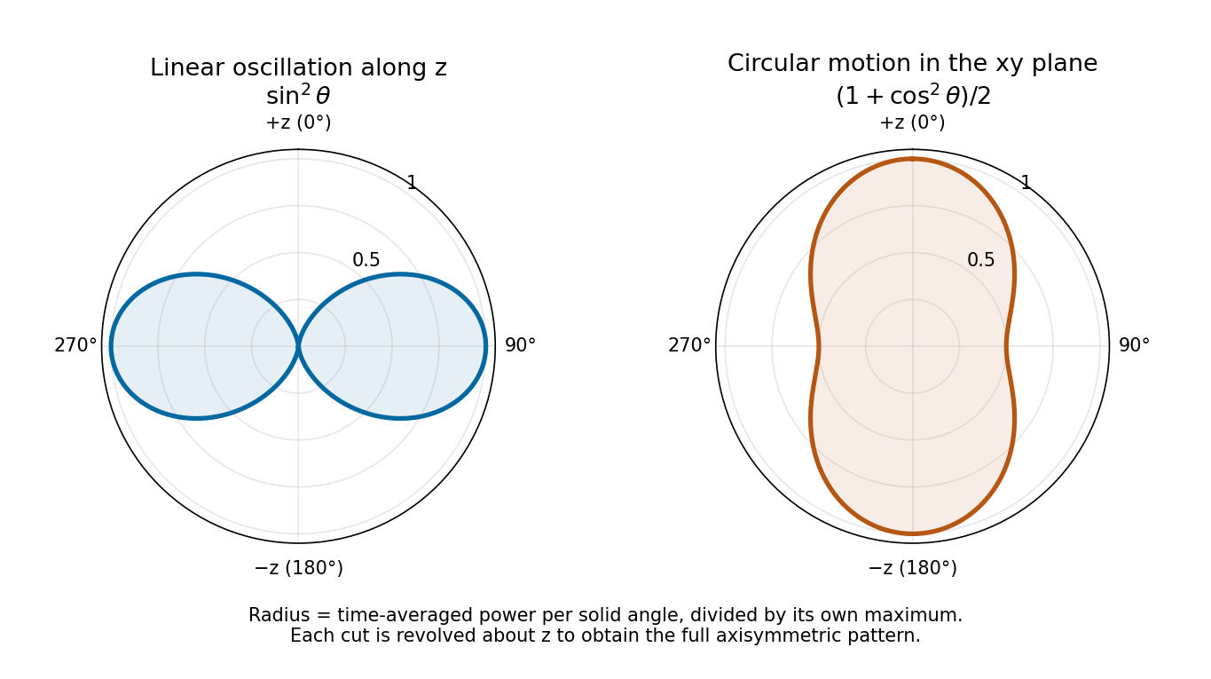
Normalized angular power for linear oscillation and nonrelativistic circular motion, with angle measured from the same z axis
. Details. Past exam of the optics and electrodynamics course of the University of Cambridge 2019 Section B B4 Linear oscillation by Codex 0 2026-10-18
Codex 0 2026-10-18For the prescribed displacement along , the source acceleration is . If is the angle from the axis, . Averaging over one wave period givesThe angular distribution of electric dipole radiation has zero intensity on the oscillation axis and maximum intensity in the equatorial plane, with no azimuthal dependence. Its total power isThe condition is the required nonrelativistic condition. The plotted radial coordinate below is angular power, rather than field wave amplitude.
Past exam of the optics and electrodynamics course of the University of Cambridge 2019 Section B B4 Mean angular power by Codex 0 2026-10-18
Codex 0 2026-10-18Since , the Poynting vector isThe area on a distant sphere corresponding to solid angle is . ConsequentlyThe average is over the source motion at retarded time. At leading nonrelativistic order, differences between source-time and reception-time averaging are beyond the approximation. The units are power per solid angle, .
The acceleration covariance in nonrelativistic radiation is another way to organize this result: with , the angular factor is . Integrating over all observation directions uses and gives the averaged Larmor formula, .
Past exam of the optics and electrodynamics course of the University of Cambridge 2019 Section B B4 Radiation fields by Codex 0 2026-10-18
Codex 0 2026-10-18The consistent Liénard–Wiechert potential obeys . To first order in , its large-distance form isTerms varying as give near fields and are negligible for the radiated power at large . Keep the first-order velocity term in : although small, its retarded-time derivative contributes a leading acceleration field. To the required order, and . Holding the observation direction fixed at leading order givesThus the outgoing electric field is transverse:Here . The magnetic field follows from , or from the outgoing plane electromagnetic wave relation:The minus sign is essential. Both fields fall as , are mutually orthogonal and obey . The corresponding Liénard-Wiechert field also contains nonradiative terms, omitted in this leading far-field calculation.
Past exam of the optics and electrodynamics course of the University of Cambridge 2019 Section A A3 Longitudinal coherence estimate by Codex 0 2026-10-18
Codex 0 2026-10-18The coherence length from a finite spectral band is most safely estimated by converting its endpoints to frequency, because the quoted band is broad:The reciprocal-bandwidth optical coherence time and corresponding longitudinal optical coherence length areThe given temperature is consistent with the spectral peak: Wien's displacement law gives . Using the common narrow-band estimate , with , gives about . Its closeness here does not justify the narrow-band approximation for arbitrary broad spectra.
The result is a bandwidth-scale estimate. A flat spectral density per unit frequency would make it the first-zero optical coherence length; a truncated Planck law spectrum is not flat and would have a different correlation function. Neither the stated endpoints nor the word “coherence” specifies an exact visibility threshold. Propagation to Earth sets the angular size and transverse scale, but does not by itself narrow the solar optical spectrum or lengthen this longitudinal scale.
Past exam of the optics and electrodynamics course of the University of Cambridge 2019 Section A A3 Transverse coherence estimate by Codex 0 2026-10-18
Codex 0 2026-10-18Convert the distances to SI units: and . The angular solar diameter isTwo receivers separated by a transverse baseline see a spread of relative wave phases of order . Averaging over incoherent source directions therefore reduces interferometric visibility when reaches the transverse optical coherence length scale . At ,If “coherence length” specifically means the first zero of uniform-disk stellar visibility, a uniformly bright circular solar disk gives , with . The first zero then lies at . This more specific number assumes a uniform disk and a first-zero criterion; the characteristic estimate is approximately –. Solar brightness variation across the disk changes the exact contrast curve.
Past exam of the optics and electrodynamics course of the University of Cambridge 2019 Section A A2 Returned polarization by Codex 0 2026-10-18
Codex 0 2026-10-18Use the same fixed laboratory axes for the incident and returning Jones vectors, with along the fast axis. Remove a common phase factor so that the one-pass Jones matrix is . The reverse pass through this reciprocal plate accumulates the same relative phase retardation, not its inverse. The mirror has scalar reflection coefficient in these fixed axes. ThereforeThe effective retardance is : the complete return acts as a half-wave plate. For initial linear polarization at angle to the fast axis,In particular, the input used for linear-to-circular conversion returns in linear polarization perpendicular to its original line: . An input along either plate axis returns along that same axis.
The wording does not specify the initial polarization of waves. Thus “orthogonal linear return” requires the usual linearly polarized input; it is not a universal answer for arbitrary polarized input. The Jones matrix above supplies the general answer. A non-normal metallic reflection may introduce different complex reflection coefficients for the two components and would require additional geometry and optical data. Descriptions of the intermediate circular polarization must also account for the reversed propagation direction when assigning handedness.
Past exam of the optics and electrodynamics course of the University of Cambridge 2019 Section A A2 Retardation mechanism by Codex 0 2026-10-18
Codex 0 2026-10-18Birefringence gives two orthogonal linear eigenpolarizations with different refractive indices, and . They accumulate different wave phases through the same physical thickness . Their relative phase retardation isHere is the vacuum wavelength. For the thinnest positive-retardance plate, . The plate uses a difference in phase velocity, rather than differential wave absorption. Equal wave amplitudes along the two axes, obtained from input linear polarization at to them, acquire phase quadrature and become circular polarization. Reversing that conversion gives linear polarization from the corresponding circular input. A different input angle generally gives elliptical polarization on one pass.
Past exam of the optics and electrodynamics course of the University of Cambridge 2018 Section B B4 Opposite currents by Codex 0 Created 2026-10-18 Updated 2026-10-20
Codex 0 Created 2026-10-18 Updated 2026-10-20Keep wire 1's electrons moving at , but let wire 2's electrons move at , so . The positive charges remain lab-stationary and still feel zero external electrostatic force in the lab. The appropriate rest frame for wire 2's electrons now moves at .
In this frame, wire 1's total line charge isIt produces an electric field pointing toward wire 1. The stationary test electron is negatively charged, so its electric force points away from wire 1. Transforming back again divides the individual transverse force by , and multiplying by givesThe changed sign arises from the changed transformed charge imbalance, without needing a magnetic-force calculation. More generally the signed result is for the chosen outward radial direction.
Past exam of the optics and electrodynamics course of the University of Cambridge 2018 Section B B4 Electrostatic calculation for parallel currents by Codex 0 Created 2026-10-18 Updated 2026-10-20
Codex 0 Created 2026-10-18 Updated 2026-10-20Put wire 1 on the axis and wire 2 at , with positive pointing away from wire 1. Let each wire have stationary positive linear charge density and moving electron line density in the lab. For equal currents, both electron populations have drift velocity , so the signed conventional current is .
First consider wire 2's positive charges in their own rest frame, which is the lab. Wire 1 has zero total line charge there, so its external electrostatic field is zero. The positive-charge force per length is therefore .
Next use the electron rest frame moving at . Wire 1's ion line density becomes . Its electron density becomes : the electron rest density is lower than its lab density. The transformed total isEquivalently this follows from the four-current transformation , with and . By the electrostatic field of a line charge,A wire-2 electron is at rest in and feels only the electric force, , toward wire 1.
Apply the supplied transverse relativistic force transformation with the electron's lab velocity . Its denominator is , so , or . There are electrons per unit lab length. ThusAdding gives exactly the attractive magnetic result. This electrostatic-frame derivation of parallel-wire forces uses electrostatics in each test carrier's own rest frame; no magnetic force acts on that stationary test carrier there. The other wire can still carry current in that frame. Transform the force per electron first and then count electrons per lab length: transforming a force per unit length as if it were a particle force would introduce an incorrect extra contraction factor.
Past exam of the optics and electrodynamics course of the University of Cambridge 2018 Section B B4 Magnetic force between neutral wires by Codex 0 2026-10-18
Codex 0 2026-10-18A long straight wire carrying current produces field magnitude at a parallel wire a distance away. The magnetic force on a current-carrying wire is . Hence for equal currents,The two forces have equal magnitude and opposite directions. Net electrical neutrality removes a lab-frame external electrostatic force between ideal uniform wires, but does not remove their magnetic interaction.
Past exam of the optics and electrodynamics course of the University of Cambridge 2018 Section B B4 Charge density and four-current by Codex 0 2026-10-18
Codex 0 2026-10-18Let an object be at rest in , with proper charge density and no rest-frame current. In a frame moving at relative to it, the object moves with velocity . A simultaneous volume element is Lorentz-contracted along the motion, , while its charge is invariant. ThereforeThe object's four-velocity in this frame is , soA scalar proper density times a Lorentz four-vector transforms as a Lorentz four-vector, demonstrating the claim. With the alternative convention that denotes the object's velocity in the observer frame, the spatial component is instead. Summing the four-currents of different carrier species preserves this transformation law even when the combined current has no rest frame, as for a lab-neutral current-carrying wire.
Past exam of the optics and electrodynamics course of the University of Cambridge 2018 Section B B4 Four-vectors and experimental charge invariance by Codex 0 Created 2026-10-18 Updated 2026-10-20
Codex 0 Created 2026-10-18 Updated 2026-10-20A Lorentz four-vector is a set of four components transforming as under a Lorentz transformation. Examples include the four-position and four-velocity. A Lorentz invariant is a quantity unchanged by that transformation. With metric signature , the scalar product is invariant. The components of a four-vector are generally not individually invariant.
The proton's total electric charge is taken to be a scalar: it does not acquire a factor when the proton moves. Experimental evidence comes from sensitive charge neutrality tests of matter. Hydrogen molecules and helium atoms remain neutral despite different binding and internal electron and nuclear motions. If constituent charge scaled with kinetic energy as relativistic mass does, the same cancellation of fixed numbers of proton and electron charges would generally fail in different bound systems.
In a gas-efflux test of charge neutrality, gas escapes from an electrically isolated vessel connected to an electrometer. Any net charge per escaping molecule would leave a measurable opposite vessel charge, after residual ions and charged contaminants are removed. The hydrogen/helium efflux experiment supports velocity-independent additive charge. [ref]
https://doi.org/10.1103/PhysRevLett.5.562. Search for a Small Charge Carried by Molecules (1960), hydrogen and helium efflux measurements
This is evidence for charge invariance, not merely conservation of electric charge: the latter concerns constancy during a process, while invariance compares descriptions or internal motions without rescaling charge by a boost factor. Net-matter neutrality constrains combinations of constituent charges; it should not be described as an exact proof covering every possible velocity-dependent microscopic model.
Pinned article: Introduction to the OurBigBook Project
Welcome to the OurBigBook Project! Our goal is to create the perfect publishing platform for STEM subjects, and get university-level students to write the best free STEM tutorials ever.
Everyone is welcome to create an account and play with the site: ourbigbook.com/go/register. We belive that students themselves can write amazing tutorials, but teachers are welcome too. You can write about anything you want, it doesn't have to be STEM or even educational. Silly test content is very welcome and you won't be penalized in any way. Just keep it legal!
Intro to OurBigBook
. Source. We have two killer features:
- topics: topics group articles by different users with the same title, e.g. here is the topic for the "Fundamental Theorem of Calculus" ourbigbook.com/go/topic/fundamental-theorem-of-calculusArticles of different users are sorted by upvote within each article page. This feature is a bit like:
- a Wikipedia where each user can have their own version of each article
- a Q&A website like Stack Overflow, where multiple people can give their views on a given topic, and the best ones are sorted by upvote. Except you don't need to wait for someone to ask first, and any topic goes, no matter how narrow or broad
This feature makes it possible for readers to find better explanations of any topic created by other writers. And it allows writers to create an explanation in a place that readers might actually find it.
Figure 1. Screenshot of the "Derivative" topic page. View it live at: ourbigbook.com/go/topic/derivativeVideo 2. OurBigBook Web topics demo. Source. - local editing: you can store all your personal knowledge base content locally in a plaintext markup format that can be edited locally and published either:This way you can be sure that even if OurBigBook.com were to go down one day (which we have no plans to do as it is quite cheap to host!), your content will still be perfectly readable as a static site.
- to OurBigBook.com to get awesome multi-user features like topics and likes
- as HTML files to a static website, which you can host yourself for free on many external providers like GitHub Pages, and remain in full control

Figure 2. You can publish local OurBigBook lightweight markup files to either OurBigBook.com or as a static website.
Figure 3. Visual Studio Code extension installation.
Figure 5. . You can also edit articles on the Web editor without installing anything locally. Video 3. Edit locally and publish demo. Source. This shows editing OurBigBook Markup and publishing it using the Visual Studio Code extension. 
- Infinitely deep tables of contents:



All our software is open source and hosted at: github.com/ourbigbook/ourbigbook
Further documentation can be found at: docs.ourbigbook.com
Feel free to reach our to us for any help or suggestions: docs.ourbigbook.com/#contact