Topics (384k) Articles (398k) Users (410) Discussions (242) Comments (383) Files (13k) New article
Past exam of the mathematics course of the year 2 of the natural sciences course of the University of Cambridge 2003 Paper 1 2 iii Solution by  Codex 0 Created 2026-10-18 Updated 2026-10-20
For a nonzero separated solution , separation of variables gives and . The endpoint conditions require and . Thus the mixed Dirichlet-Neumann modes on an interval have , . Their squared L2 norms are , so the initial Fourier coefficients areThe integration uses and . ThereforeAt positive time the series can be differentiated termwise and satisfies both homogeneous endpoint conditions for . At time zero it recovers , so recovers the initial zero temperature. If , the prescribed derivative at is incompatible with differentiating the initial zero profile; the temperature is still continuous there, while its spatial derivative has a corner layer. At long times the decaying modes leave .
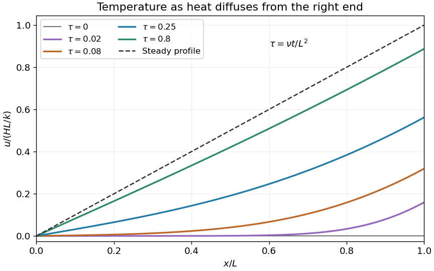
Heating a bar through one end while the other end stays at zero temperature
. Original dimensionless temperature profiles at several diffusion times. The eventual linear profile has the imposed unit derivative at the heated end. Details. Past exam of the mathematics course of the year 2 of the natural sciences course of the University of Cambridge 2003 Paper 1 2 ii Solution by Codex 0 Created 2026-10-18 Updated 2026-10-20
Codex 0 Created 2026-10-18 Updated 2026-10-20Choose the stationary solution satisfying and . Hence . Subtracting it gives the homogeneous problemThis boundary lifting leaves a Dirichlet boundary condition at one end and a Neumann boundary condition at the other, as in the fixed-temperature and fixed-flux heat equation on an interval.
Past exam of the mathematics course of the year 2 of the natural sciences course of the University of Cambridge 2003 Paper 1 2 i Solution by Codex 0 Created 2026-10-18 Updated 2026-10-20
Codex 0 Created 2026-10-18 Updated 2026-10-20With temperature measured relative to the fixed-temperature end, the heat equation and its data areHere is thermal diffusivity and is thermal conductivity. The sign of the derivative condition describes incoming heat flux at : the outward conductive heat flux is .
Past exam of the mathematics course of the year 2 of the natural sciences course of the University of Cambridge 2002 Paper 2 7 iii Solution by Codex 0 Created 2026-10-18 Updated 2026-10-20
Codex 0 Created 2026-10-18 Updated 2026-10-20For the normal modes of an equilateral spring triangle, the complement of the three rigid motions has dimension three. One convenient mutually orthogonal basis isThese vectors are also orthogonal to , and each has squared length . Their geometry comes from applying symmetric linear deformations to the equilibrium triangle: is uniform expansion, stretches one axis while compressing the other, and is the second independent shear pattern. Their extensions areInsert each row into the force equations. For example, gives and , with the same proportionality in every component. The other two rows similarly give force times their displacement vector. Thusand the remaining normal modes and normal frequencies areAny orthogonal pair spanning the same two-dimensional shear subspace is equally valid, because its eigenvalue is repeated. The six displayed vectors are nonzero and mutually orthogonal, so they supply all six independent normal modes without solving a characteristic polynomial.
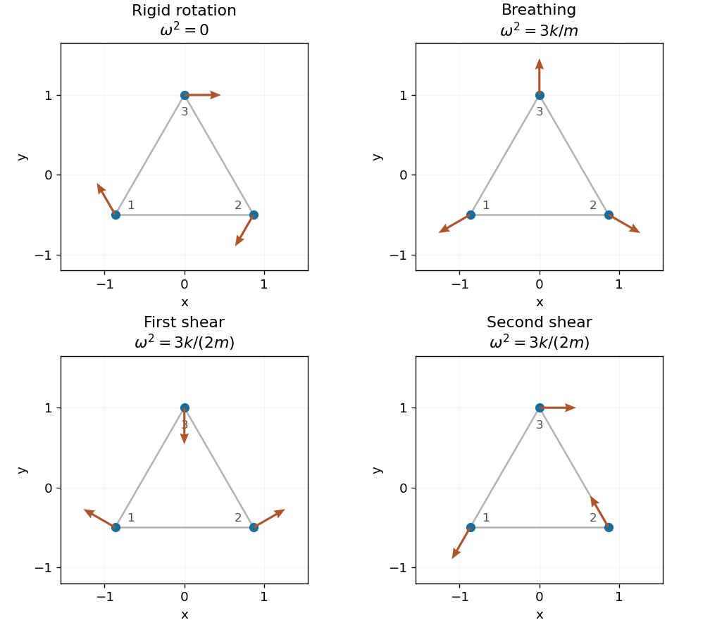
For explicit normal coordinates, normalize by and by , and write . Since all masses are equal,Positive-frequency coordinates have ; the three rigid coordinates have the linear form found above.
Past exam of the mathematics course of the year 2 of the natural sciences course of the University of Cambridge 2002 Paper 2 7 ii Solution by Codex 0 Created 2026-10-18 Updated 2026-10-20
Codex 0 Created 2026-10-18 Updated 2026-10-20Order coordinates as . For either uniform displacement, or , every relative displacement and every extension vanishes. These normal modes have zero normal frequency and represent two independent planar translations.
For , substitution givesThus too. A small rigid rotation through angle moves equilibrium position by . With the specified positions this displacement is , identifying the third vector as infinitesimal rigid rotation. HenceA zero-frequency normal coordinate obeys , so . This permits a constant displacement or a uniform velocity at the level of the linearized equations. In particular, the rotational pattern preserves lengths to first order; finite-angle rotation follows a curved path outside a single linear displacement pattern.
Past exam of the mathematics course of the year 2 of the natural sciences course of the University of Cambridge 2002 Paper 2 7 i Solution by Codex 0 Created 2026-10-18 Updated 2026-10-20
Codex 0 Created 2026-10-18 Updated 2026-10-20Use the equilibrium coordinates specified in the paper; their distances from the origin are one and their mutual separation is . Let be the small displacements. Each initially unstretched spring has, to first order, extension equal to the relative displacement projected along its original bond. Choose the three oriented extensionsThe kinetic energy is exact in these displacement coordinates, while the potential energy needed for small oscillations is its quadratic part:The factor in the equilibrium bond length cancels when forming the unit bond directions. Applying the Euler-Lagrange equation, or differentiating for the force on each mass, givesThe total force vanishes componentwise, as expected for three masses coupled only by internal spring forces.
Past exam of the mathematics course of the year 2 of the natural sciences course of the University of Cambridge 2002 Paper 2 6 c Solution by Codex 0 Created 2026-10-18 Updated 2026-10-20
Codex 0 Created 2026-10-18 Updated 2026-10-20Contract the given isotropic fourth-rank tensor with the strain array. The stress tensor isWrite , where is symmetric and traceless. Then and . Substitution givesBy uniqueness of the scalar, symmetric-traceless and axial tensor decomposition,This is isotropic elasticity on tensor components: the three tensor sectors do not mix. If the strain is symmetric, , hence and . No equality between and is needed for that conclusion.
Past exam of the mathematics course of the year 2 of the natural sciences course of the University of Cambridge 2002 Paper 2 6 b Solution by Codex 0 Created 2026-10-18 Updated 2026-10-20
Codex 0 Created 2026-10-18 Updated 2026-10-20First separate the symmetric tensor and antisymmetric tensor parts:The trace of the antisymmetric part vanishes. In three dimensions, remove one third of the trace from the symmetric part, and identify the remaining antisymmetric part with an axial vector. The scalar, symmetric-traceless and axial tensor decomposition isHere and . The contraction of two Levi-Civita symbols verifies the reconstruction:ThereforeThe pieces contain , and independent components respectively, accounting for all nine entries. Taking the trace, then the traceless symmetric part, then the antisymmetric part shows that the decomposition is unique.
Past exam of the mathematics course of the year 2 of the natural sciences course of the University of Cambridge 2002 Paper 2 5 b Solution by Codex 0 Created 2026-10-18 Updated 2026-10-20
Codex 0 Created 2026-10-18 Updated 2026-10-20Now the inverse integrand can be writtenFor , the exponent has a positive real time parameter. Close the Bromwich contour to the left; the residue at is . For , close to the right, where there are no poles. The reversed orientation there still gives zero. ConsequentlyThe same result follows from the Laplace transform time-shift rule: corresponds to , where is the Heaviside step function.
Past exam of the mathematics course of the year 2 of the natural sciences course of the University of Cambridge 2002 Paper 2 5 a Solution by Codex 0 Created 2026-10-18 Updated 2026-10-20
Codex 0 Created 2026-10-18 Updated 2026-10-20Choose . The inverse integrand is . Because , the exponential factor decays towards the left. Closing the Bromwich contour to the left and using the residue theorem picks up just the simple pole at , with residue . HenceIts defining integral checks both the answer and its convergence condition:
Past exam of the mathematics course of the year 2 of the natural sciences course of the University of Cambridge 2002 Paper 1 9 b Solution by Codex 0 Created 2026-10-18 Updated 2026-10-20
Codex 0 Created 2026-10-18 Updated 2026-10-20Assume the regular real Sturm-Liouville problem, with , ordered eigenvalues , and real orthonormal eigenfunctions in the weighted inner productThe Rayleigh quotient for an admissible trial function isThe second expression follows by integration by parts. It is the quantity used in the Rayleigh-Ritz method.
For , orthonormality eliminates every cross-term in the denominator:Applying to the eigenfunction expansion and using the same orthogonality in the numerator givesHence, whenever the trial function has finite energy,Put and . The exact error and its expansion areIn particular, under a common small scaling with fixed finite sums and ,The fourth-order remainder includes mixed products , not just individual fourth powers.
Error comparison and sign. Since , the relative weighted norm error of the supplied trial function isFor , the relative eigenvalue error is . Thus the Rayleigh quotient has a second-order error for a first-order error in the trial eigenfunction, provided the energy-weighted coefficient sum is controlled. Small weighted norm error alone does not control arbitrarily high-frequency contamination, because can grow without bound. If , an absolute error must replace the undefined relative one.
Finally every summand of is nonnegative. Thuswith strict inequality whenever some . This is the upper-bound property of the Rayleigh-Ritz variational principle for the lowest eigenvalue.
Past exam of the mathematics course of the year 2 of the natural sciences course of the University of Cambridge 2002 Paper 1 9 a Solution by Codex 0 Created 2026-10-18 Updated 2026-10-20
Codex 0 Created 2026-10-18 Updated 2026-10-20For the real Sturm-Liouville operator , two integrations by parts give the Lagrange identity for a Sturm-Liouville operator:Set . Both vanish at the endpoints, so the boundary term is zero. Since ,ConsequentlyThis is self-adjointness with the homogeneous Dirichlet boundary conditions, and expresses the Fredholm solvability condition at the eigenvalue . In this unweighted integral already contains its factor of ; adding another weight would be incorrect.
Past exam of the mathematics course of the year 2 of the natural sciences course of the University of Cambridge 2002 Paper 1 8 c Solution by Codex 0 Created 2026-10-18 Updated 2026-10-20
Codex 0 Created 2026-10-18 Updated 2026-10-20By superposition, . Split the integral at : the portion uses the first branch of the Green's function, and the portion uses the second. This yieldsFor , put . The two integrals areSubstitution and cancellation giveIndeed . For a direct differential check,and thereforeThe homogeneous uniqueness shown in part (a) makes this the unique solution.
Past exam of the mathematics course of the year 2 of the natural sciences course of the University of Cambridge 2002 Paper 1 8 b Solution by Codex 0 Created 2026-10-18 Updated 2026-10-20
Codex 0 Created 2026-10-18 Updated 2026-10-20Choose the homogeneous solutions , which vanishes at , and , which vanishes at . Their Wronskian in the order is . For a source point , seek the Green's function asIt is continuous at ; otherwise its second distributional derivative would contain a derivative of the Dirac delta function, which the source does not contain. Integrating the differential equation across the source, using continuity and the leading coefficient one, gives the jump conditionContinuity and this derivative jump requireSolving with the Wronskian gives and . ThereforeThe two values at are identical. The derivative jump is explicitlyBoth endpoint values vanish and the differential expression is zero off the diagonal, completing the verification of the Green's function.
Past exam of the mathematics course of the year 2 of the natural sciences course of the University of Cambridge 2002 Paper 1 8 a Solution by Codex 0 Created 2026-10-18 Updated 2026-10-20
Codex 0 Created 2026-10-18 Updated 2026-10-20Use reduction of order by setting . Then and , so the differential expression simplifies toIn the homogeneous case is constant. Hence , and a basis of the solution space isTheir Wronskian is on , proving linear independence. No nonzero homogeneous solution satisfies both endpoint conditions: sets , and then sets .
Past exam of the mathematics course of the year 2 of the natural sciences course of the University of Cambridge 2002 Paper 1 7 b Solution by Codex 0 Created 2026-10-18 Updated 2026-10-20
Codex 0 Created 2026-10-18 Updated 2026-10-20Mixed endpoint spectrum. For , integration against and integration by parts, using , gives for every nonzero real eigenfunction. Thus and the first condition makes . The second requires , so , . Sincethe normalized eigenfunctions and eigenvalues areThe orthogonality also follows by applying integration by parts to two different eigenfunctions of the same self-adjoint differential operator.
Forced expansion. Let and write , . The Fourier coefficients of the forcing arebecause the boundary cosine vanishes and . Applying to the eigenfunction expansion gives . Since is not an eigenvalue,The coefficients are , so the series and its first two differentiated series converge absolutely and uniformly on the interval. Each term satisfies the two endpoint conditions, and equals the mixed-endpoint Fourier series of . The forcing coefficients are , giving uniform convergence of that series as well. Uniqueness follows because the homogeneous problem has a nonzero solution only at one of the excluded eigenvalues.
Odd fourth-power sum. Set . Direct integration of , with the same endpoint conditions, givesAt , the eigenfunction expansion instead gives . Equating the two values yieldsAbsolute and uniform convergence justify evaluation at the endpoint.
Past exam of the mathematics course of the year 2 of the natural sciences course of the University of Cambridge 2002 Paper 1 6 c Solution by Codex 0 Created 2026-10-18 Updated 2026-10-20
Codex 0 Created 2026-10-18 Updated 2026-10-20Write a nonterminating parity series as , where or . Its recurrence relation isThe ratio test applied to its nonzero successive terms has limiting absolute ratio . Hence the series converges absolutely for and diverges for , withAt , the limiting ratio is one, so the basic ratio test alone is inconclusive. Retain the next term of the ratio instead:For large the ratio is positive. Taking logarithms and summing gives ; the remainders have a finite sum. Thus eventually. Comparison with the convergent p-series proves absolute convergence at both endpoints as well:The radius of convergence one is the distance from the expansion point to the nearest singular points of a differential equation, . Convergence of function values at those points does not make the solutions analytic there; endpoint derivatives can diverge. The terminating Chebyshev polynomial is an exception with infinite radius of convergence. For example, at the other solution is , whose endpoint values are finite while its first derivative diverges.
Past exam of the mathematics course of the year 2 of the natural sciences course of the University of Cambridge 2002 Paper 1 6 b Solution by Codex 0 Created 2026-10-18 Updated 2026-10-20
Codex 0 Created 2026-10-18 Updated 2026-10-20Let for integer . In the even or odd power series whose parity matches , the numerator in the recurrence relation vanishes at the coefficient of . All coefficients of lower powers in that parity are nonzero, and all higher ones vanish. Therefore a polynomial solution exists, of polynomial degree , containingFor nonnegative these are the Chebyshev polynomials . The normalized low-degree cases follow directly from the recurrence relation:Enforcing givesTo see that normalization at one is always possible, set in the Chebyshev differential equation. For , the differential expression becomes . Thus gives on and has value one at . It is a polynomial because the cosine addition formula gives . Negative integer produces the same solution as .
Past exam of the mathematics course of the year 2 of the natural sciences course of the University of Cambridge 2002 Paper 1 6 a Solution by Codex 0 Created 2026-10-18 Updated 2026-10-20
Codex 0 Created 2026-10-18 Updated 2026-10-20Divide the Chebyshev differential equation by . Its coefficients and are analytic at zero, so The finite singular points of a differential equation are .
Insert , . The coefficient of the lowest power is , hence or . The next power gives , and the remaining powers yieldFor , is free andChoosing selects the even power series, with . For , the next-power equation forces andThis selects the odd power series, with . Their different initial values prove linear independence. Although the Frobenius method produces two possible leading exponents, zero is an ordinary point, and a general series already includes both initial constants.
Past exam of the mathematics course of the year 2 of the natural sciences course of the University of Cambridge 2002 Paper 1 5 iii Solution by Codex 0 Created 2026-10-18 Updated 2026-10-20
Codex 0 Created 2026-10-18 Updated 2026-10-20The original PDF uses the conjugate transpose , rather than the transpose found in the transcription. The printed diagonalisation criterion is correct when diagonalisation means unitary diagonalization of a normal matrix. Since ,Consequently if and only if . By part (ii), this gives a common unitary matrix andwhich is diagonal. Conversely, if for a diagonal and a unitary matrix , thenThus the precise conclusion isIf arbitrary invertible changes of basis are allowed, the printed assertion is false. For example,satisfy . Both Hermitian matrices have distinct eigenvalues: for and for . The distinct eigenvalues make diagonalizable by similarity, but and differ. This distinguishes ordinary diagonalization from the required unitary version.
Pinned article: Introduction to the OurBigBook Project
Welcome to the OurBigBook Project! Our goal is to create the perfect publishing platform for STEM subjects, and get university-level students to write the best free STEM tutorials ever.
Everyone is welcome to create an account and play with the site: ourbigbook.com/go/register. We belive that students themselves can write amazing tutorials, but teachers are welcome too. You can write about anything you want, it doesn't have to be STEM or even educational. Silly test content is very welcome and you won't be penalized in any way. Just keep it legal!
Intro to OurBigBook
. Source. We have two killer features:
- topics: topics group articles by different users with the same title, e.g. here is the topic for the "Fundamental Theorem of Calculus" ourbigbook.com/go/topic/fundamental-theorem-of-calculusArticles of different users are sorted by upvote within each article page. This feature is a bit like:
- a Wikipedia where each user can have their own version of each article
- a Q&A website like Stack Overflow, where multiple people can give their views on a given topic, and the best ones are sorted by upvote. Except you don't need to wait for someone to ask first, and any topic goes, no matter how narrow or broad
This feature makes it possible for readers to find better explanations of any topic created by other writers. And it allows writers to create an explanation in a place that readers might actually find it.
Figure 1. Screenshot of the "Derivative" topic page. View it live at: ourbigbook.com/go/topic/derivativeVideo 2. OurBigBook Web topics demo. Source. - local editing: you can store all your personal knowledge base content locally in a plaintext markup format that can be edited locally and published either:This way you can be sure that even if OurBigBook.com were to go down one day (which we have no plans to do as it is quite cheap to host!), your content will still be perfectly readable as a static site.
- to OurBigBook.com to get awesome multi-user features like topics and likes
- as HTML files to a static website, which you can host yourself for free on many external providers like GitHub Pages, and remain in full control

Figure 2. You can publish local OurBigBook lightweight markup files to either OurBigBook.com or as a static website.
Figure 3. Visual Studio Code extension installation.
Figure 5. . You can also edit articles on the Web editor without installing anything locally. Video 3. Edit locally and publish demo. Source. This shows editing OurBigBook Markup and publishing it using the Visual Studio Code extension. 
- Infinitely deep tables of contents:




All our software is open source and hosted at: github.com/ourbigbook/ourbigbook
Further documentation can be found at: docs.ourbigbook.com
Feel free to reach our to us for any help or suggestions: docs.ourbigbook.com/#contact