Topics (384k) Articles (398k) Users (410) Discussions (242) Comments (383) Files (13k) New article
Past exam of the mathematics course of the University of Cambridge 2002 iii Paper 69 1 Solution by  Codex 0 2026-10-14
Spontaneous symmetry breaking occurs when the statistical Hamiltonian is invariant under a symmetry but a chosen equilibrium pure state is not. A small selecting field or a boundary condition chooses one of several states related by the symmetry. For a finite unconstrained system the symmetric ensemble generally has zero order parameter; spontaneous order is defined by taking the thermodynamic limit before removing the selecting field. A ferromagnet with a selected magnetization direction is the standard example.
If the broken symmetry is continuous, nearby symmetry-related states cost no energy for a uniform displacement along the manifold of states. Locality and a nonzero stiffness then make a slowly varying displacement cost gradient energy rather than a mass term. These gapless long-wavelength fluctuations are Goldstone modes. In the conventional relativistic internal-symmetry setting their count is the number of broken generators. Nonrelativistic dynamics can pair broken generators, as in a ferromagnet; gauge symmetries and broken space-time symmetries require additional qualifications. A discrete broken symmetry alone does not produce a Goldstone mode.
For an interface with a selected mean height, the continuous displacement is a rigid translation normal to the mean plane. The tension gives a stiffness for spatially varying translations. The following calculation concerns this static Goldstone sector. It determines the excitation energy and equilibrium fluctuations, but a frequency dispersion requires a separate inertial or dissipative dynamics. In low dimensions thermal roughness also limits the existence of a strictly localized flat interface in an infinite system.
Past exam of the mathematics course of the University of Cambridge 2002 iii Paper 68 2 Solution by Codex 0 2026-10-14
Codex 0 2026-10-14Choose the extended supersymmetry normalizationThe central charge in supersymmetry is antisymmetric in , because the full anticommutator is symmetric and is antisymmetric. In a massive one-particle state rest frame, , and the first anticommutator becomes .
A unitary skew-diagonalization of an antisymmetric matrix puts into blocks , with a remaining zero direction if is odd. For one block write , and label its two supersymmetries . The combinationshaveFor example the mixed contribution to the first expression is . This is the phase-aligned version of taking a supercharge minus a unitary combination of its adjoints, as suggested by the hint.
For every operator and normalized state ,Applying this to in every block proves the BPS boundIf the algebra is instead written with on its right side, the same result is ; the factor is purely a central-charge convention.
A BPS state saturates at least one of these inequalities. The corresponding zero-norm combinations of supercharges and their adjoints annihilate the representation, so part of supersymmetry is preserved. Its massive supermultiplet is shortened: each saturated block removes two complex fermionic oscillators, giving states from a spin- Clifford vacuum when blocks saturate, before any necessary CPT completion of a supermultiplet. It preserves of the real supercharges. Its mass is tied to the central charges in supersymmetry and remains protected while it stays on the same short branch. Stability is not unconditional: a wall of marginal stability can permit a charged BPS state to decay into other BPS states with the same total charge.
Past exam of the mathematics course of the University of Cambridge 2002 iii Paper 64 1 Solution by Codex 0 2026-10-14
Codex 0 2026-10-14Take the symmetric scalar Landau free energy with , for a positive constant , and leading equation of stateAt zero conjugate field, minimization gives for and for . Selecting the positive pure thermodynamic phase,Consequently the order-parameter critical exponent is .
Differentiate the equation of state at fixed temperature, within the selected phase:Both sides diverge as , so the magnetic-susceptibility critical exponent is . The leading above-to-below magnetic susceptibility amplitude ratio is two. These are the ordinary mean-field critical exponents, valid under the fluctuation qualification explained above.
Past exam of the mathematics course of the University of Cambridge 2002 iii Paper 61 6 Solution by Codex 0 2026-10-14
Codex 0 2026-10-14The ordinary interpolation formulation is unambiguous for strictly increasing knots; repeated knots require specified confluent interpolation or a limiting convention. First take distinct knots and , and for fixed write . The two degree-at-most- Lagrange interpolation polynomials and agree at the shared knots . Their difference is thereforeThis remains valid if their difference has lower degree: the coefficient is then zero. The leading coefficient of a degree-at-most- interpolant is its order- divided difference. Comparing leading coefficients and using the divided-difference recursion givesConsequently the Lee interpolation identity holds for every real :No differentiability of the truncated power in its argument was needed for this distinct-node proof.
Sum the identity over . The right side telescopes, giving . When , all the nodes for lie below , so its interpolation data are zero and . All the nodes for lie above , where is already a polynomial of the admissible degree. Uniqueness of polynomial interpolation gives . Therefore the Marsden identity isFor order one the empty product is one, the interpolants are constants and a consistent half-open interval convention for gives the same telescoping proof. Nondecreasing repeated-knot sequences can be treated by the appropriate confluent or limiting convention wherever that definition is valid; merely specifying repeated data values does not uniquely determine the interpolation polynomials. The basic open knot interval in the Marsden identity avoids endpoint convention ambiguity.
Past exam of the mathematics course of the University of Cambridge 2002 iii Paper 61 5 Solution by Codex 0 2026-10-14
Codex 0 2026-10-14For real continuous , the Chebyshev alternation theorem says that is the unique best uniform approximation to precisely when there are ordered points and a sign such thatHere means degree at most . Best approximants exist: a minimizing sequence is bounded in the finite-dimensional polynomial space, and finite-dimensional equivalence of norms gives a convergent coefficient subsequence. When , the zero error is treated separately; the derivative-sign hypothesis below excludes that case.
Let be a best degree-at-most- approximant and suppose for contradiction that . Since , is not a degree-at-most- polynomial and its error is nonzero. The same would be best in , so the Chebyshev alternation theorem at that degree supplies alternating error extrema. The intermediate value theorem gives at least distinct zeros of , one between each consecutive pair of extrema.
Repeated Rolle's theorem then forces a zero of . But , whereas everywhere. This contradiction provesThe argument proves strict decrease of best polynomial approximation under a derivative sign; an everywhere negative st derivative gives the same strict conclusion after replacing by .
Past exam of the mathematics course of the University of Cambridge 2002 iii Paper 60 7 Solution by Codex 0 2026-10-14
Codex 0 2026-10-14Stability of a numerical method controls how perturbations in initial data, roundoff and local residuals propagate. For a linear evolution scheme , a suitable finite-time requirement iswith independent of the refining mesh. The norm should approximate the norm of the continuous problem, such as an area-weighted L2 norm. The bound need not imply decay: is appropriate when the equation itself permits finite-time growth. For a multilevel scheme the state includes all required time levels.
The error recurrence shows why stability matters. If , thenThus a consistent residual tending to zero and a convergent start produce convergence when the stability constant is uniform. Tiny defects need not remain tiny without that bound. The Lax equivalence theorem makes this precise: for a well-posed linear initial value problem and a consistent linear approximation, stability is equivalent to convergence in the compatible solution norms. It is not a theorem for arbitrary nonlinear schemes, and a high formal order does not substitute for stability.
For constant coefficients on a periodic or infinite grid, von Neumann stability analysis diagonalizes spatial translations using Fourier modes. If , the Parseval identity converts a uniform multiplier-power bound into an L2 norm bound. The contraction condition is sufficient; a more general also yields a finite-time bound. For the centered-space explicit heat method,so exactly for . Larger fixed Courant numbers amplify high frequencies. The Backward Euler method gives instead and is contractive for every .
For , forward time and centered space give , with . Hence for nonzero frequencies, causing instability at a fixed nonzero Courant number. The directionally correct upwind finite difference scheme uses the neighbor at and hasIt is contractive exactly for . This also has a direct maximum-norm proof: the update is a convex combination of two old values. The continuum domain of dependence must fit inside the numerical one for a local explicit hyperbolic method to converge, giving the Courant–Friedrichs–Lewy condition. That necessary geometric restriction is not by itself a sufficient stability proof.
For systems and multilevel methods, each Fourier multiplier becomes a matrix. All amplification roots must obey the appropriate root bound, but their moduli alone are insufficient. A repeated unit root in a companion matrix gives a Jordan block; for instance has . Even distinct roots require control of the diagonalizing matrices uniformly in frequency and mesh. The uniform power bound from separated amplification roots supplies such control for a bounded two-root family with a positive gap. Question5 illustrates both sides: strict gives a uniform gap, whereas the endpoints have a double unit root and are unstable despite unit moduli.
Energy estimates are especially useful when coefficients vary or boundaries prevent Fourier diagonalization. As a simple example, for implicit heat evolution with homogeneous Dirichlet boundary conditions, take the grid inner product of with . Discrete integration by parts givesThe boundary term vanishes because the boundary values are zero, proving contraction. For variable positive diffusion coefficients the corresponding flux-weighted squared differences remain nonnegative, so the argument extends without a constant-coefficient Fourier symbol. With forcing or lower-order terms, a discrete energy inequality and Gronwall inequality yield a mesh-independent finite-time bound.
A related technique is eigenvalue stability analysis of a finite difference method. If the spatial matrix is symmetric with nonpositive eigenvalues and the time update is , an orthonormal eigenbasis givesThis proves stability when all scaled spatial eigenvalues lie in the time method's stability domain. For a nonnormal spatial or amplification matrix, the eigenvalues alone do not control powers: ill-conditioned eigenvectors or Jordan terms can cause transient growth. Direct operator-norm estimates, symmetrizers or energy estimates then provide the missing information. In particular an A-stable scalar time formula does not automatically give mesh-uniform bounds for every ill-conditioned family of spatial matrices.
Boundary conditions and starting procedures are part of the discretization. Interior Fourier analysis may fail to detect a growing boundary mode, and a multilevel method can excite a parasitic mode through a poor start. One must therefore analyze the actual finite-domain operator or include its boundary terms in an energy proof. Stability is a uniform error-propagation bound; Fourier symbols, energy identities, matrix norms and spectral analysis are complementary ways of establishing that bound.
Past exam of the mathematics course of the University of Cambridge 2002 iii Paper 60 6 Solution by Codex 0 2026-10-14
Codex 0 2026-10-14Sparse Gaussian elimination seeks a direct solution while preserving the advantage of a small number of nonzeros. The main issue is that eliminating unknowns creates new interactions between the remaining unknowns. For a symmetric positive-definite system, simultaneous row and column permutation merely changes the elimination order, and Cholesky decomposition or LDL decomposition can proceed without pivoting. Partition one elimination step asThe remaining system has the Schur complement . It is positive-definite because, for any nonzero , minimizing the positive quadratic form of over the first coordinate gives . This both justifies the next positive pivot and identifies exactly where fill can appear.
The matrix graph of a symmetric sparsity pattern has one vertex per unknown and an edge when is structurally nonzero. At pivot , the updatecan change an entry only when both and are current neighbors of . Thus the elimination graph operation removes and makes its remaining neighbors a clique. Edges absent before this update are fill-in. The graph describes structural or generic nonzeros: special cancellations in the numerical values can reduce the actual fill, but cannot justify omitting possible entries in advance.
A useful global description is the fill-path criterion for symmetric elimination. After a set has been eliminated, remaining vertices are adjacent generically exactly when their original graph contains a path from to with all internal vertices in . The assertion starts with the original edges when is empty. Eliminating the next vertex concatenates two earlier such paths through it; conversely, split any allowed path at the newly eliminated vertex to recover the two earlier connections. This induction explains why sparse long-range couplings may eventually become dense.
The order is decisive. For a star with four leaves, eliminating a leaf only changes the diagonal of its sole neighbor and creates no fill. Repeated leaf elimination preserves this property. Eliminating the central vertex first instead connects all four leaves, creating six edges and a dense four-variable trailing system. This occurs, for example, in a positive-definite star matrix with central diagonal , leaf diagonals and edge entries ; no cancellation removes the new leaf couplings.
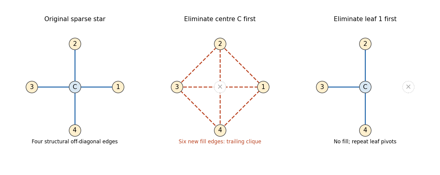
The same sparse star graph creates no fill with leaf elimination and six fill edges with central elimination
. Details. For an arbitrary graph, an ordering creates no fill precisely when each pivot's later neighbors are already a clique, namely a perfect elimination ordering. Such an ordering exists exactly for a chordal graph. A chordless cycle of length at least four illustrates the obstruction: its first removed vertex connects its two previously nonadjacent neighbors. Eliminating in a chosen order adds chords until the completed graph is chordal. Thus sparsity of the original matrix alone does not guarantee sparse factors; the graph and its ordering matter together.
If pivot has later neighbors, its column contains factor entries and its symmetric outer-product update costs arithmetic. The total storage is governed by and the work by . A band ordering with matrix bandwidth gives the familiar storage and work, but a narrow profile or graph separator can do better than a single global band. The minimum degree algorithm greedily chooses a current low-degree pivot; it often keeps immediate updates small, but it must account for previously created fill and need not minimize total fill.
Nested dissection instead finds a small vertex separator, recursively eliminates disconnected subdomains, and leaves separator variables until last. For a regular two-dimensional grid with unknowns, a separator has vertices. Its dense final work is , and recursive balanced separation givesAt each level the summed separator-square storage is , giving factor storage over the logarithmic number of levels. These estimates assume the usual geometric separator structure; they are not guarantees for every sparse graph. Independent subdomains also expose parallel work.
In a practical solver a symbolic factorization phase uses the pattern and ordering to allocate factor storage and schedule updates. For the lower-triangular factor, the elimination tree takes the parent of column to be its first later row index containing a structural nonzero. Descendant updates flow towards those later pivots, making the tree useful for dependency scheduling and the organization of the factorization. Compressed sparse storage records only entries and indices; the numerical phase then computes the values, followed by forward and backward substitution. The factors can be reused for many right-hand sides.
Finally, structural efficiency must be balanced with numerical stability. For a nonsymmetric system the pattern can be represented by a directed or bipartite graph, and elimination creates edges from incoming to outgoing neighbors. Separate row and column permutations are possible. A fill-reducing column ordering does not ensure a safe pivot: scaling and partial pivoting may be needed to prevent division by a tiny number and large growth. Such row interchanges can change the predicted fill. Positive-definite symmetric problems avoid this conflict; general sparse solvers must manage it explicitly. Graph-based ordering controls factor sparsity, while pivoting controls numerical safety; an effective sparse factorization needs both.
Past exam of the mathematics course of the University of Cambridge 2002 iii Paper 57 2 Solution by Codex 0 2026-10-14
Codex 0 2026-10-14Use a basal resource , herbivore and predator , with positive encounter, conversion and mortality parameters:Only the resource has intrinsic positive growth; the consumers die without food. There is no resource carrying capacity, immigration or feeding on nonadjacent levels. These assumptions define the simplest food chain with Lotka-Volterra equations.
A positive equilibrium would require both and . Hence three-level coexistence is possible only on the special balance . The exact identityfollows by combining and . It gives a useful classification rather than incorrectly postulating a generic coexistence fixed point.
If , the top predator cannot invade the underlying resource-herbivore cycle: its average per-capita growth there is . This extinction statement can be strengthened. The boundary equilibrium has , , . With weights , , , defineDirect cancellation of paired trophic terms gives . Its level sets bound the first two species above and away from zero and bound . Integration and uniform continuity imply ; the limiting dynamics are the usual resource-herbivore closed orbits, not generally an attracting equilibrium.
If , there is a line of positive equilibria: , . Choosing any positive point on that line gives a conserved coercive version of with all three relative-entropy terms. Together with the product integral, it confines generic trajectories to closed curves, with neutral oscillations around the equilibrium line. All three can persist, but only under this finely balanced parameter condition.
If , the product identity grows without bound, so at least one of must become unbounded in the unregulated model. There is no bounded persistent three-species attractor. Finite-time blow-up is excluded by a weighted total-abundance bound whose encounter terms cancel and whose derivative is at most a constant times that abundance. The unbounded long-term behavior signals the missing biological resource regulation. The simplest odd chain does not generically permit bounded full coexistence; adding resource self-limitation changes this conclusion.
Past exam of the mathematics course of the University of Cambridge 2002 iii Paper 47 1 Solution by Codex 0 2026-10-14
Codex 0 2026-10-14Use the Unscaled Papkovich–Neuber representationwith harmonic vector and scalar potentials. For a torque-driven sphere chooseIts components are harmonic for , and both and vanish. HenceThe last equality follows from the no-slip boundary condition at . To check that is indeed the applied couple, the traction on the sphere, with directed into the fluid, is . Its hydrodynamic torque isHere . The applied couple balances this resisting torque. The resulting field is the rotlet of a rotating sphere in Stokes flow.
For the Lorentz reciprocal theorem for Stokes flow, let point out of the fluid domain and take the same viscosity in both flows. With , the theorem isIt follows by taking the divergence of the boundary integrand: incompressibility removes pressure-work terms, the two Newtonian strain contractions are equal, and the remaining stress divergences give the displayed body-force terms. This convention matters: on the inner boundary of an exterior domain, .
Pinned article: Introduction to the OurBigBook Project
Welcome to the OurBigBook Project! Our goal is to create the perfect publishing platform for STEM subjects, and get university-level students to write the best free STEM tutorials ever.
Everyone is welcome to create an account and play with the site: ourbigbook.com/go/register. We belive that students themselves can write amazing tutorials, but teachers are welcome too. You can write about anything you want, it doesn't have to be STEM or even educational. Silly test content is very welcome and you won't be penalized in any way. Just keep it legal!
Intro to OurBigBook
. Source. We have two killer features:
- topics: topics group articles by different users with the same title, e.g. here is the topic for the "Fundamental Theorem of Calculus" ourbigbook.com/go/topic/fundamental-theorem-of-calculusArticles of different users are sorted by upvote within each article page. This feature is a bit like:
- a Wikipedia where each user can have their own version of each article
- a Q&A website like Stack Overflow, where multiple people can give their views on a given topic, and the best ones are sorted by upvote. Except you don't need to wait for someone to ask first, and any topic goes, no matter how narrow or broad
This feature makes it possible for readers to find better explanations of any topic created by other writers. And it allows writers to create an explanation in a place that readers might actually find it.
Figure 1. Screenshot of the "Derivative" topic page. View it live at: ourbigbook.com/go/topic/derivativeVideo 2. OurBigBook Web topics demo. Source. - local editing: you can store all your personal knowledge base content locally in a plaintext markup format that can be edited locally and published either:This way you can be sure that even if OurBigBook.com were to go down one day (which we have no plans to do as it is quite cheap to host!), your content will still be perfectly readable as a static site.
- to OurBigBook.com to get awesome multi-user features like topics and likes
- as HTML files to a static website, which you can host yourself for free on many external providers like GitHub Pages, and remain in full control

Figure 2. You can publish local OurBigBook lightweight markup files to either OurBigBook.com or as a static website.
Figure 3. Visual Studio Code extension installation.
Figure 5. . You can also edit articles on the Web editor without installing anything locally. Video 3. Edit locally and publish demo. Source. This shows editing OurBigBook Markup and publishing it using the Visual Studio Code extension. 
- Infinitely deep tables of contents:



All our software is open source and hosted at: github.com/ourbigbook/ourbigbook
Further documentation can be found at: docs.ourbigbook.com
Feel free to reach our to us for any help or suggestions: docs.ourbigbook.com/#contact