Topics (384k) Articles (398k) Users (410) Discussions (242) Comments (383) Files (13k) New article
Past exam of the mathematics course of the University of Cambridge 2003 iii Paper 17 5 Solution by  Codex 0 2026-10-14
A compatible almost complex structure is a smooth endomorphism satisfying , preserving , and making a positive-definite inner product. Preservation and make this bilinear form symmetric.
To construct one, choose any Riemannian metric and define by . The endomorphism is skew-adjoint and invertible. Consequently is positive definite and self-adjoint. Let be its positive square root and setThe spectral theorem gives fibrewise, and the positive-square-root operation is smooth on positive-definite matrices, so this defines a smooth endomorphism. Since commutes with , . Also , so . Commutation then givesThis is the metric construction of a compatible almost complex structure, proving nonemptiness.
If we start with for an already compatible , then , so , , and the construction recovers . For two compatible structures, linearly interpolate their metrics,and apply the construction to . This is a continuous smooth-in- path with endpoints . Thus the space is nonempty and path connected. Interpolating instead to a single fixed auxiliary metric actually gives the contractibility of compatible almost complex structures.
Past exam of the mathematics course of the University of Cambridge 2003 ib Paper 2 4E Solution by Codex 0 2026-10-14
Codex 0 2026-10-14For the cofinite topology , the empty set and are included. A nonempty union of cofinite sets is cofinite because its complement is contained in the finite complement of any one member. A finite intersection is cofinite because its complement is a finite union of finite sets; intersections involving the empty set are empty. This proves all topology axioms.
For the tail topology on the natural numbers , . Any nonempty collection of tails has a smallest starting index, so its union is that tail; a finite intersection of tails is the tail with largest starting index. Empty sets and empty-family conventions supply the remaining cases. Thus is also a topology.
We classify continuous maps between cofinite and tail topologies. Continuity is equivalent toIf has unbounded image, each is nonempty, hence cofinite. For every threshold , eventually , which is exactly . If the image is bounded, it is a nonempty finite subset of and has a maximum . Then is nonempty and cofinite, but always, so except at finitely many indices. These exhaust the two possibilities and prove necessity. Their sufficiency is checked separately below.
Past exam of the mathematics course of the University of Cambridge 2003 ia Paper 4 7C Solution by Codex 0 2026-10-14
Codex 0 2026-10-14For integers not both zero, their greatest common divisor is the greatest positive integer dividing both. For the degenerate pair use the conventional value zero. A number divides both exactly when it divides both : one direction uses closure of divisibility under sums; the reverse subtracts . The positive common-divisor sets are therefore identical, provingThis also holds for under the stated convention and does not depend on the signs of the integers.
Bezout identity states that there exist integers such that . If a prime divides but does not divide , then , so choose with . Multiplying by gives . Both terms on the left are divisible by , so . Thuswhich proves the Euclid lemma from the requested identity. The separately numbered entries use these arithmetic facts for the Fibonacci numbers.
Past exam of the mathematics course of the University of Cambridge 2003 ia Paper 4 2C Solution by Codex 0 2026-10-14
Codex 0 2026-10-14An equivalence relation on a set is a binary relation that is reflexive, symmetric and transitive: every satisfies ; implies ; and , imply . Each of these quantifiers ranges over the entire specified set. The separate entries below test these three properties.
Past exam of the mathematics course of the University of Cambridge 2003 ia Paper 2 7D Solution by Codex 0 2026-10-14
Codex 0 2026-10-14For the homogeneous solution, expand in the independent eigenvectors of . Each coefficient obeys , so the complementary function isIf is any particular integral, subtracting it from any other solution gives a homogeneous solution. Hence is the general solution. Complex-conjugate modes can be combined to produce real solutions when the forcing is real.
For a real two-by-two matrix, the characteristic polynomial is . Under the stated distinct-eigenvalue assumption, all nonzero homogeneous modes are purely oscillatory exactly when the eigenvalues are with . Their sum and product imply , . Conversely these trace and determinant conditions force those eigenvalues, so there is no exponential growth, decay or Jordan-block secular growth.
For the final specified initial-value problem, direct multiplication gives . The forcing vector satisfies , so the forcing is resonant and is a particular integral. The matrix exponential isSince the resonant particular integral vanishes initially, the initial-value solution isThis complex solution is appropriate to the complex forcing as written. Taking real parts gives the corresponding solution for the real part of that forcing.
Past exam of the mathematics course of the University of Cambridge 2003 ia Paper 2 1D Solution by Codex 0 2026-10-14
Codex 0 2026-10-14The direction field has slope , independent of . Its line segments slope upward for , are horizontal at , and slope downward for . Thus is an attracting equilibrium in forward , while is repelling. The two constant solutions must be included separately when separating variables.
The following original sketch shows the slope field and one solution in each requested region. The lower exterior solution ends at a finite pole; it cannot be continued across that pole as a real finite-valued solution.
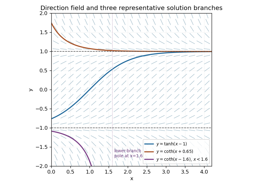
Direction field, equilibrium lines and representative solutions in the three regions of the autonomous scalar equation
. Details. Past exam of the mathematics course of the University of Cambridge 2003 ia Paper 1 8D Solution by Codex 0 2026-10-14
Codex 0 2026-10-14Two nonzero vectors are linearly independent when implies . Their span then has dimension two. If they are linearly dependent, one is a scalar multiple of the other, so their span is a nonzero line and has dimension one. Thus the requested dimensions are two and one, respectively.
The dot product and corresponding Euclidean norm areThe Cauchy-Schwarz inequality states . If this is immediate. Otherwise the nonnegativity of a squared norm, with , givesMultiplying by and taking square roots proves the inequality. Equality holds precisely when the vectors are linearly dependent. Expanding another squared norm and using the inequality givesand hence the triangle inequality .
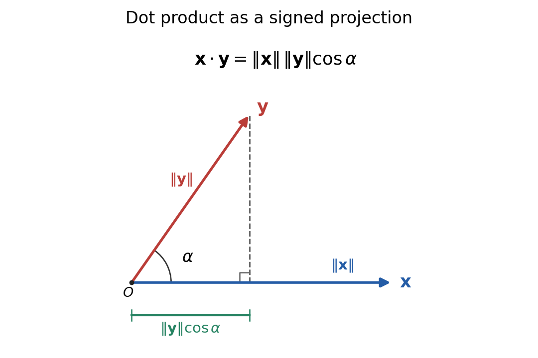
In , the two vectors lie in a common plane. If their directions make angle , the law of cosines gives . Comparing with the dot-product expansion yieldsThe sketch shows the same relation as a projection: multiply the length of by the signed component of in its direction. That component is negative for obtuse .
A unit vector is a vector of Euclidean norm one, equivalently . In particular the dot product of two unit vectors is the cosine of their mutual angle.
Past exam of the mathematics course of the University of Cambridge 2003 ia Paper 1 7B Solution by Codex 0 2026-10-14
Codex 0 2026-10-14There are nontrivial proper normal subgroups. The determinant defines a surjective group homomorphism . Its kernel is the rotational symmetry group of a cube, a normal subgroup of order twenty-four. Also is a central subgroup of order two: central inversion preserves the cube and commutes with every matrix. Both provide affirmative examples.
For the body diagonal through , write a general cube symmetry as , with a permutation matrix and , each . Since , preserving the unoriented diagonal requires to be either or . ThusThe map from to is a group homomorphism, because central inversion commutes with every coordinate permutation. It is surjective by the displayed description and injective because a permutation matrix cannot equal the negative of another permutation matrix. Consequently the body-diagonal stabilizer in the cube symmetry group isThis also agrees with the orbit-stabilizer theorem for the transitive action on the four body diagonals. The line is preserved as a set, so exchanging its opposite endpoints is allowed.
Past exam of the mathematics course of the University of Cambridge 2003 ia Paper 1 4C Solution by Codex 0 2026-10-14
Codex 0 2026-10-14The radius of convergence of a power series is the unique for which the series converges absolutely when and diverges when . When it converges for every complex ; when it converges only at the centre. The definition makes no assertion about convergence on , so boundary points must be checked separately.
Past exam of the mathematics course of the University of Cambridge 2003 ia Paper 1 10F Solution by Codex 0 2026-10-14
Codex 0 2026-10-14The integral test for convergence applies when for all sufficiently large , where is nonnegative, continuous and nonincreasing on . It states that converges if and only if the improper integral is finite. Its comparison bounds areNo conclusion about an arbitrary nonnegative sequence follows without such a monotone comparison function; finite initial terms do not affect convergence.
For with , all the hypotheses hold. If ,whereas for the integral is . The first expression has a finite limit exactly when . Thus the p-series satisfies
Past exam of the mathematics course of the University of Cambridge 2002 iii Paper 8 5 Solution by Codex 0 2026-10-14
Codex 0 2026-10-14For , write for the coordinates other than , and setBy Tonelli theorem, . The key estimate is the functional Loomis-Whitney inequality:Here is a proof in every dimension. In dimension two, the left-hand side separates into a product of two one-dimensional integrals, so Tonelli theorem gives equality. For , first integrate . Apply Hölder's inequality with factors to , which may depend on , and leave the factor outside that integral. WriteEach depends on the coordinates other than . With , the full integral is at mostPut . A second application of Hölder's inequality, with exponents and , bounds this expression byBy induction in dimension , . Since , substitution proves the claimed functional inequality. Nonnegative integrands justify all integrations; truncation gives the extended-valued version if necessary.
The pointwise hypotheses imply , soApply the proved functional inequality and take the power to obtainFor the useful case all the right-hand norms are finite. If one of them is zero, its line integral vanishes for almost every transverse coordinate and forces almost everywhere; there is no division by that factor. In dimension one the corresponding direct assertion is .
Past exam of the mathematics course of the University of Cambridge 2002 iii Paper 76 3 Solution by Codex 0 2026-10-14
Codex 0 2026-10-14Let contain all free variables of . The lambda term is a solvable lambda term if there are closed lambda terms such thatAdditional arguments beyond the first are allowed. A head normal form is a term with a variable at the head; its arguments need not be beta-normal.
If reduces to this head normal form, close its free variables and supply every resulting initial binder with the same closed projection(take when ). The head variable becomes and discards all argument terms, even divergent ones, leaving . Thus a head normal form implies solvability.
Conversely suppose a closure and applications of yield . The standardization theorem for beta reduction supplies a finite successful head-reduction sequence. Until exposes a head variable, its head contractions lie within : a closing substitution cannot create a new head redex there, and supplied arguments cannot be used until an initial abstraction is exposed. Each such contraction commutes with the closing capture-avoiding substitution. Project the successful head computation back onto , ignoring contractions in supplied arguments and the consumption of its initial binders. If this projected head computation did not reach a variable-headed spine, the full computation could not reach either. It therefore gives a finite head reduction of to a head normal form. ConsequentlyThe same head-trace argument shows that an unsolvable lambda term stays unsolvable under substitution and application. This also justifies the unsolvability conclusion in the preceding solution.
Past exam of the mathematics course of the University of Cambridge 2002 iii Paper 72 1 Solution by Codex 0 2026-10-14
Codex 0 2026-10-14Use sequential semicolon indices: , where the second covariant derivative also differentiates the lower index of . For a torsion-free connection, direct expansion givesSubtract the expression with exchanged. Commuting partial derivatives cancel the first term; the first-derivative terms cancel in pairs; symmetry of the lower Christoffel symbol indices cancels both terms containing . What remains isThis is the Ricci identity with the curvature convention printed on the PDF's first page. In terms of derivative operators it is ; writing the operator order explicitly avoids reversing the sign.
The lower-index rule follows by applying the commutator to the scalar contraction . Its second derivatives commute, so the product rule implies . The derivative commutator is a derivation on tensor products, since the cross terms cancel. It therefore acts once on every index, with a positive sign on each upper index and a negative sign on each lower index. For an arbitrary tensor of valence ,Local sums of decomposable tensors establish the formula for every tensor field, rather than only for a single tensor product.
Past exam of the mathematics course of the University of Cambridge 2002 iii Paper 69 2 Solution by Codex 0 2026-10-14
Codex 0 2026-10-14The renormalization group compares descriptions at successively longer length scales. First eliminate short-wavelength degrees of freedom, then rescale coordinates and fields to restore the reference cutoff. This changes the couplings, including interactions and additive free-energy terms generated during elimination. A renormalization-group fixed point is a scale-invariant description. Linearized directions growing under coarse graining are relevant, shrinking directions are irrelevant, and zero-eigenvalue directions are marginal and require higher-order analysis.
A diverging correlation length means that many coarse-graining steps can approach a renormalization-group fixed point before a relevant perturbation becomes large. Systems with different microscopic details but the same renormalization-group fixed point and relevant directions share universal critical behavior. For the quadratic model below, Fourier modes decouple, so eliminating a high-momentum shell produces a Gaussian determinant but does not couple the remaining modes. The anisotropic gradient kernel requires different length rescalings in the parallel and transverse directions. This is an anisotropic renormalization group, not an isotropic rescaling of all coordinates.
Pinned article: Introduction to the OurBigBook Project
Welcome to the OurBigBook Project! Our goal is to create the perfect publishing platform for STEM subjects, and get university-level students to write the best free STEM tutorials ever.
Everyone is welcome to create an account and play with the site: ourbigbook.com/go/register. We belive that students themselves can write amazing tutorials, but teachers are welcome too. You can write about anything you want, it doesn't have to be STEM or even educational. Silly test content is very welcome and you won't be penalized in any way. Just keep it legal!
Intro to OurBigBook
. Source. We have two killer features:
- topics: topics group articles by different users with the same title, e.g. here is the topic for the "Fundamental Theorem of Calculus" ourbigbook.com/go/topic/fundamental-theorem-of-calculusArticles of different users are sorted by upvote within each article page. This feature is a bit like:
- a Wikipedia where each user can have their own version of each article
- a Q&A website like Stack Overflow, where multiple people can give their views on a given topic, and the best ones are sorted by upvote. Except you don't need to wait for someone to ask first, and any topic goes, no matter how narrow or broad
This feature makes it possible for readers to find better explanations of any topic created by other writers. And it allows writers to create an explanation in a place that readers might actually find it.
Figure 1. Screenshot of the "Derivative" topic page. View it live at: ourbigbook.com/go/topic/derivativeVideo 2. OurBigBook Web topics demo. Source. - local editing: you can store all your personal knowledge base content locally in a plaintext markup format that can be edited locally and published either:This way you can be sure that even if OurBigBook.com were to go down one day (which we have no plans to do as it is quite cheap to host!), your content will still be perfectly readable as a static site.
- to OurBigBook.com to get awesome multi-user features like topics and likes
- as HTML files to a static website, which you can host yourself for free on many external providers like GitHub Pages, and remain in full control

Figure 2. You can publish local OurBigBook lightweight markup files to either OurBigBook.com or as a static website.
Figure 3. Visual Studio Code extension installation.
Figure 5. . You can also edit articles on the Web editor without installing anything locally. Video 3. Edit locally and publish demo. Source. This shows editing OurBigBook Markup and publishing it using the Visual Studio Code extension. 
- Infinitely deep tables of contents:




All our software is open source and hosted at: github.com/ourbigbook/ourbigbook
Further documentation can be found at: docs.ourbigbook.com
Feel free to reach our to us for any help or suggestions: docs.ourbigbook.com/#contact