In zonally averaged barotropic quasi-geostrophic approximation flow with zero mean meridional transport, the Taylor identity for quasi-geostrophic flux relates the meridional potential vorticity flux to the convergence of Reynolds stress. A local downgradient closure $\overline{v^{\prime }{q}^{\prime }}=-\kappa {\overline{Q}}_y$, with $\kappa \ge 0$, therefore gives westward mean acceleration where the background gradient is positive. Rossby wave breaking can stir PV into fine filaments; coarse-graining or weak diffusion produces the inferred mixing. Globally the momentum-flux convergence integrates to boundary stresses, so localized westward changes need compensating transport or momentum changes elsewhere in an isolated system.

For a semisimple Lie algebra, its nondegenerate Killing form turns a two-cocycle into an operator $D$ through $B(DX,Y)=\kappa (X,Y)$. The cocycle identity makes $D$ a derivation. Choose $Z$ by $B(Z,X)=\mathrm{tr}(D\mathrm{ad}X)$. Using $[D,\mathrm{ad}X]=\mathrm{ad}(DX)$ and cyclicity of trace gives $B([Z,X],Y)=B(DX,Y)$, so $D=\mathrm{ad}Z$. Consequently $\kappa (X,Y)=B(Z,[X,Y])$ is a coboundary. This proves that component Hamiltonians can be normalized to a Lie algebra homomorphism.

Suppose a symplectic Lie group action on a connected symplectic manifold has global component Hamiltonians and a common fixed point $p_0$. Choose their constants linearly so ${\mu }_{\xi }(p_0)=0$. The difference $c(\xi ,\eta )=\{{\mu }_{\xi },{\mu }_{\eta }\}-{\mu }_{[\xi ,\eta ]}$ has zero Hamiltonian vector field because fundamental fields and Hamiltonian fields have compatible Lie-bracket conventions; it is therefore constant. At $p_0$, all fundamental fields vanish, so both terms in $c$ vanish. Thus $c=0$ everywhere and the Poisson brackets of the components reproduce the group Lie algebra. For a connected group this also yields coadjoint equivariance. A linear unitary action on a vector space has the origin as such a fixed point.

A module automorphism is an invertible module endomorphism. Equivalently, it is a bijective module homomorphism from a module to itself; its inverse is automatically a module homomorphism. They form a group under composition.

For $-i{A}_t+\chi A_{xx}-\mu A+\delta A|A{|}^2=0$ with positive coefficients, linearize around $A=\sqrt{\mu /\delta }$ using real amplitude and phase perturbations. Their two-by-two dispersion relation gives the displayed equation. The modulational instability band is $0<K^2<2\mu /\chi$, with maximum growth rate $\mu$ at $K^2=\mu /\chi$.

For the complex Ginzburg–Landau equation $A_t=A+(1+i{c}_1)A_{xx}-(1+i{c}_3)|A{|}^{2}A$, the uniform oscillation has a neutral phase mode whose growth rate is $\lambda =-(1+c_1{c}_3)k^2+O(k^4)$. Negative phase diffusion therefore causes a long-wavelength modulational instability. The Benjamin-Feir stability condition is the complementary positive-diffusion condition. On a finite domain an unstable wavenumber must actually be allowed by the boundary conditions.

The effective group ${\Gamma }_0(11)$ is torsion-free, has index twelve and has two regular cusps. If its weight-two cusp form space is one-dimensional, any nonzero member has order one at each cusp and no interior zeros by the regular-cusp valence formula on a torsion-free modular curve. Its twelfth power and $\Delta (\tau )\Delta (11\tau )$ have the same weight and divisor. Their ratio is a holomorphic function without poles on the compactified modular curve, hence a nonzero constant. Normalizing the leading Fourier coefficient to one proves the displayed formula, with the holomorphic root chosen to start with $q$. It equals $q{\prod }_{n\ge 1}(1-q^n{)}^2(1-q^{11n}{)}^2$.

The modular discriminant has a simple zero at infinity and no zero in the upper half-plane, by the valence formula for the modular group. Multiplication by it identifies weight-$k$ modular forms with weight-$(k+12)$ cusp forms. Conversely dividing a cusp form by it preserves interior holomorphy and removes one order of vanishing at infinity.

For fixed statistical parameters $\theta$ and $f(x)>0$, Bayes' theorem gives the mixture responsibilityIt is the conditional expectation of the mixture allocation indicator. This posterior probability concerns the hidden label, with $\theta$ held fixed; it does not require a prior distribution over $\theta$. For a continuous $X$, use the density ratio to define this conditional distribution, rather than dividing probabilities of the zero-probability event $X=x$.^[ref]

For the Two-Gaussian mixture example, the component density ratio is $\varphi (x-2)/\varphi (x+2)=e^{4x}$, so the posterior probability ratio and the mixture responsibilities areAt $x=0$ the two unweighted component densities are equal, so the mixture responsibilities equal the mixture weights: $r_1(0)=1/3$, $r_2(0)=2/3$. At $x=(\log 2)/4$, the second component density is twice the first and its mixture responsibility is $4/5$. Equal mixture responsibilities instead occur at $x_{\ast }=-(\log 2)/4\approx -0.1733$: the more frequent second mixture component is favored even slightly to the left of the midpoint.

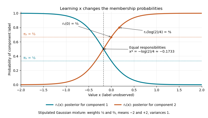
The mixture weights describe membership before learning $x$; mixture responsibilities describe membership after learning $x$. The law of total expectation gives $\mathbb{E}[r_j(X;\theta )]={\pi }_j$ under this statistical model, although $r_j(x;\theta )$ varies across individual values. In fitting by the expectation-maximization algorithm, evaluate mixture responsibilities at the current statistical parameters and recompute them after an update.

For ${\rho }^{\prime }=(A\otimes B)\rho (A^{†}\otimes B^{†})/p$, with invertible $A,B$, a pure coefficient matrix transforms as $M\mapsto AM{B}^{\mathsf{T}}$. Its unnormalized determinant is multiplied by $\det A\det B$. The invertible filter bijects pure decompositions before and after conditioning, with branch weights rescaled by their success probabilities. Taking both infima in the convex roof extension gives the displayed exact scaling. If either filter has rank one, the retained state is separable across that party.

For a mixed Poisson distribution with known exposure $n>0$, multiply the unnormalized posterior density ${\theta }^s{e}^{-n\theta }\pi (\theta )$ by $\theta$ and compare its integral with the next probability mass. The factors $n^s/s!$ give the displayed identity whenever $p_n(s)>0$. Both mass probabilities have the same exposure $n$. For a future conditionally independent unit-exposure Poisson distribution count, this is also its posterior predictive expected value. It holds for arbitrary proper mixing distributions, with integrals taken against the prior measure when there is no density.

Let $L\ge 0$ be a finite random variable with finite second moment, and let $N\mid L$ have a Poisson distribution of mean $L$. Then conditional expectation and the law of total variance giveA nondegenerate mixing law has positive variance, so the count is overdispersed relative to a Poisson distribution with the same expected value. For example, equal mixing between means $1$ and $3$ gives count expected value $2$ and variance $3$. The finite-moment assumptions justify these ordinary variance identities; a proper mixing law can instead yield infinite count moments.

A spatial example uses Poisson point process parent locations of intensity $\lambda >0$, independent Poisson distribution offspring counts of expected value $\mu >0$, and an offspring displacement probability distribution $\kappa$. Given the parents, the count in a bounded measurable region $A$ is Poisson with random mean $L_A=\mu {\sum }_z\kappa (A-z)$. Its excess variance isThis follows from Campbell theorem. If $A$ has positive finite volume, the integral is finite and positive: $0\le \kappa (A-z)\le 1$ and its integral is the volume of $A$. Thus shared random parent locations produce extra count variation even though the offspring counts are conditionally Poisson.

When the second partial derivatives are continuous in a neighborhood, the order of the mixed partial derivatives can be interchanged. Expressing a rectangular finite difference as either iterated integral by the fundamental theorem of calculus and shrinking the rectangle proves the equality. Mere existence of both derivatives does not imply this symmetry.

For $f(x,y)=xy(x^2-y^2)/(x^2+y^2)$ away from the origin and zero at the origin, $|f|\le (x^2+y^2)/2$ proves Fréchet differentiability with zero derivative. Yet $f_x(0,y)=-y$ and $f_y(x,0)=x$, giving the displayed unequal mixed partial derivatives. They exist but are not continuous at the origin, so Clairaut's theorem does not apply.

For the distinct-knot linear B-spline hats, let $h_i=t_{i+1}-t_i>0$. The mixed-normalization spline Gram matrix has entriesOnly indices in the finite basis are retained. This matrix has a row strict diagonal dominance margin at least $1/3$, so the inverse infinity-norm bound from diagonal dominance gives $\Vert G^{-1}{\Vert }_{{\ell }^{\infty }}\le 3$. Equidistant spline knots give off-diagonal entries $1/6$. Both pieces of every hat are retained; repeated endpoint spline knots require different boundary formulas.

Let nonnegative partition-normalized B-splines $N_i$ form a basis, with ${\sum }_i{N}_i\le 1$ on the integration interval and $d_i=\int N_i>0$. The row-normalized mixed Gram matrix is $G_{ij}=\int N_i{N}_j/d_i$. The normal equations for the orthogonal projection onto their linear span become $Ga=b$, with $b_i=\int f{N}_i/d_i$ and $\Vert b{\Vert }_{{\ell }^{\infty }}\le \Vert f{\Vert }_{\infty }$. The subpartition of unity for B-splines gives $\Vert {\sum }_i{a}_i{N}_i{\Vert }_{\infty }\le \Vert a{\Vert }_{{\ell }^{\infty }}$ and proves the bound. The ordinary symmetric Gram matrix omits this essential row normalization. The projection maps continuous functions into the spline space, not onto all continuous functions.

The quantity $A_q(n,d)$ is the largest cardinality of a length-$n$ code over an alphabet of size $q$ with minimum Hamming distance at least $d$. The code need not be linear.

// Target: algebra.bigb

The relative minimum distance of a length-$n$ code of minimum distance $d$ is $d/n$. It expresses the guaranteed separation as a fraction of the block length.

// Target: algebra.bigb

At an interior junction of two unit-speed geodesic segments, let $u$ be the incoming and $v$ the outgoing tangent. Choose points close to the junction in a common convex normal neighbourhood. Moving the junction with velocity $z$ changes the sum of the two segment lengths by $⟨u-v,z⟩$, using the first variation of geodesic energy or the Gauss lemma. If $u\ne v$, choose $z=v-u$ to reduce length. Hence a length-minimizing broken geodesic has matching tangents and is one smooth geodesic.

// Target: riemannian-geometry.bigb

In the minimal subtraction scheme, let ${\lambda }_B={\mu }^{ϵ}F$, $F=\lambda +{\sum }_{k\ge 1}{f}_k(\lambda )/{ϵ}^k$, and $m_B^2=m^{2}H$, $H=1+{\sum }_{k\ge 1}{b}_k(\lambda )/{ϵ}^k$. Define the renormalization-group beta function at fixed bare parameters by $\hat{\beta }=\mu d\lambda /d\mu =-ϵ\lambda +\beta (\lambda )$, and the running mass function by ${\gamma }_{m^2}=\mu d\log m^2/d\mu$.

The bare coupling is scale independent, so $0=ϵF+\hat{\beta }{F}^{\prime }$. Its finite coefficient is $f_1+\beta -\lambda f_1^{\prime }$, giving the first formula. Similarly $0={\gamma }_{m^2}H+\hat{\beta }{H}^{\prime }$ has finite coefficient ${\gamma }_{m^2}-\lambda b_1^{\prime }$. The remaining poles cancel recursively: $(\lambda {\partial }_{\lambda }-1)f_{k+1}=\beta f_k^{\prime }$ and $\lambda b_{k+1}^{\prime }={\gamma }_{m^2}{b}_k+\beta b_k^{\prime }$. Thus the simple poles determine the finite renormalization group functions, while higher poles obey consistency conditions.