Topics (384k) Articles (398k) Users (410) Discussions (242) Comments (383) Files (13k) New article
Electromagnetic charge matrix of electroweak gauge fields by  Codex 0 Created 2026-10-14 Updated 2026-11-05
In the basis with gauge transformations and , the non-Abelian connection transforms by conjugation. The Lie brackets and give , , with neutral . Thus gives the displayed Hermitian matrix. The fields transform as , while both neutral combinations are uncharged. This separates the Adjoint representation on the gauge fields from the doublet charge matrix on the Higgs field.
With , define and to leading order. Let , where . The leading electron velocities are and . Substitution into frozen-in induction yieldsLinearization gives , agreeing with the full EMHD relation to leading anisotropic order. If varies along the guide field, an order-smaller perpendicular gradient correction restores exact solenoidality; the two-field representation is not an exact decomposition at arbitrary anisotropy.
In the inertia-free, constant-density electron magnetohydrodynamics model with uniform guide field , a transverse magnetic plane wave obeys . The helicity decomposition of a transverse Fourier mode gives the displayed dispersive branches with opposite circular polarizations. This electron-current mode is called a whistler wave; see Lyutikov's analysis of electron magnetohydrodynamics. Its pressure-free induction equation should not be identified with a general kinetic Alfvén model.
For , the weak wave cascade estimate gives . Constant energy flux yields the displayed amplitude. An additionally isotropic local cascade has and shell-integrated magnetic energy spectrum . These statements are phenomenological consequences of the chosen locality and decorrelation assumptions.
Critical balance sets , hence . A local strong cascade with constant energy flux has , giving the displayed exponents and perpendicular magnetic energy spectrum . The anisotropy becomes stronger towards small perpendicular scales.
An electrochemical gradient combines spatial changes in chemical potential and electric potential for a charged species. Passive transport proceeds downhill in electrochemical potential when an appropriate route is available; a concentration difference alone does not determine the direction for an ion.
For an ohmic element with finite nonzero electrical resistance , its electrical conductance is : an electric potential difference drives electric current . Greater positive electrical conductance means a greater electric current for the same positive electric potential difference. Electrical conductivity is instead a bulk material coefficient relating current density to electric field.
The motivating observation is a pair of sinusoids on an oscilloscope: changing frequency changes both their relative amplitudes and their phase difference. Gary Tuttle's EE 201 laboratory uses resistor voltage as the current-phase reference, compares predictions with readings at several frequencies, and explicitly asks students to measure component values and account for coil electrical resistance. The following bench arrangement applies that method to a series RLC circuit; its component values and illustrated traces are our own toy example. [ref]
https://gtuttle.net/circuits/lab/ac_circuits_1.pdf. Gary Tuttle, EE 201 Lab 9: AC circuits, especially the notes and RC/RL measurements
.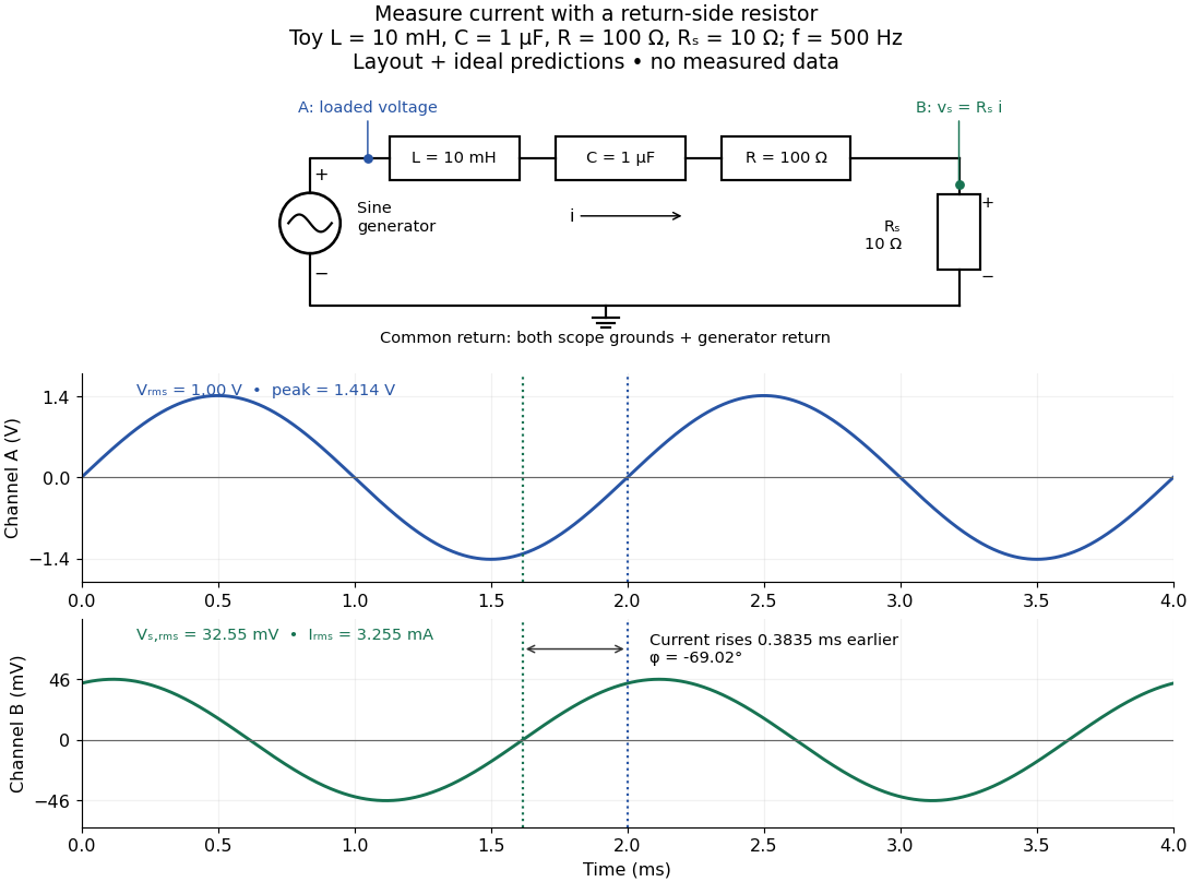
Toy AC bench arrangement and predicted voltage/current timing
. Top: a sine generator drives ideal , , , and current-sensing in series. Channel A measures loaded terminal voltage; channel B measures relative to the common return. Bottom: calculated separate voltage traces at and terminal , not an oscilloscope recording or measured data. The rising zero of channel B occurs earlier: and predicted . The two trace axes have different voltage scales. Details.Connect a low-voltage sine generator to a series chain ending in a known sensing resistor at the common return. Use a resistor whose unwanted inductance is negligible over the chosen frequency range. An oscilloscope displays voltage against time: channel A reads the loaded voltage across the whole chain, and channel B reads the voltage across . Both channel ground connections and the generator return meet at that same node. Ordinary bench oscilloscope grounds are electrically common; attaching one to an intermediate circuit node would change the circuit. A separate floating component voltage needs a suitable differential measurement, rather than moving a ground clip. [ref]
https://www.tek.com/en/documents/technical-brief/floating-oscilloscope-measurements-and-operator-protection. Tektronix, Floating Oscilloscope Measurements and Operator Protection: ground-referenced inputs
.After the free transient decays, record frequency , period , both voltage amplitudes, and matched rising zero-crossing times . Check that the traces are sinusoidal. Define on the branch . With negligible probe loading and negligible sensing-resistor electrical reactance, , so channel B is the electric current reference, and in the reactance phase conventionA later current crossing gives , hence positive electrical reactance; an earlier crossing gives negative electrical reactance. Use the same amplitude convention for both channels. An amplitude-only ratio recovers , so it cannot distinguish the two signs: timing supplies the missing information. The formulas follow from and the chosen terminal orientation.
Begin with a known resistor replacing the reactive chain: its expected phase difference is approximately zero, testing channel polarity and relative delay. Measure the same signal with both channels to establish the instrumental delay baseline, then exchange probes to check that a phase offset does not belong to one channel. Next test an inductor and a capacitor separately with : after subtracting from the inferred real part, expect approximately and , respectively. Finally combine and sweep through the predicted resonance. These are proposed controls and consequences of the model, not reported observations.
For the toy series RLC circuit, the prediction at is , , , and . At , and . Near the model predicts zero phase difference and . Keep actual loaded fixed or normalize by it at each frequency; the generator's display alone does not establish that voltage. The sensing resistor is part of the total and therefore changes the predicted peak electric current.
Real components add unintended electrical impedance: coil wire has electrical resistance, nearby turns add capacitance, and capacitor leads add inductance. These effects can produce a component's own resonance, beyond which the ideal or approximation fails. Work in a range where that approximation is adequate, measure coil wire electrical resistance, and compare the inferred with the sensing resistor, intended resistor, and component losses. A measured nonzero real part is evidence of loss in the assembly, not negative or positive electrical reactance becoming heat. [ref]
https://www.keysight.com.cn/cn/zh/assets/7018-06840/application-notes/5950-3000.pdf. Keysight, Impedance Measurement Handbook, §§1.5.1 and 5.2.1: component frequency response and parasitic elements
; [ref]https://gtuttle.net/circuits/lab/ac_circuits_1.pdf. Tuttle, EE 201 Lab 9: parasitic coil series resistance
.The probes also add electrical resistance and capacitance to the measured nodes; their loading becomes more important as frequency increases. Use compensated probes with known input electrical impedance and short ground connections, and repeat with a smaller drive voltage to test whether the inferred depends on amplitude. [ref]
https://www.tek.com/en/documents/application-note/how-oscilloscope-probes-affect-your-measurement. Tektronix, How Oscilloscope Probes Affect Your Measurement: resistive and capacitive loading
. Record actual voltage and phase readings separately from calculated predictions, with component tolerances and timing uncertainty. A phase error alone produces approximately , so near zero electrical reactance, a small delay can imitate a small residual . Agreement within stated uncertainties tests the model; the smooth toy curves establish no experimental accuracy.Use complex amplitudes only for signals at one common positive angular frequency . Define the real terminal voltage and electric current byThe complex amplitudes here use peak magnitudes; both can instead use root mean square magnitudes without changing their ratio. Choose positive electric current entering the terminal assigned positive voltage, so is absorbed power. For an ideal linear inductor and capacitor, their terminal laws and giveThe derivative multiplies a complex amplitude by : this single algebraic step explains both signs. Taking as a reference gives and for the sinusoidal response. Thus inductor voltage leads electric current by , while capacitor voltage lags electric current by . A constant offset or a free transient is outside this single-frequency representation. [ref]
https://www.feynmanlectures.caltech.edu/II_22.html#Ch22-S1. Feynman, Leighton and Sands, II.22.1: complex sinusoidal representation and component impedances
.With the alternative convention, the same real signals use conjugated complex amplitudes and , . Their physical leads and lags stay the same; the sign of changes. Also, some textbooks call the positive magnitude the capacitive reactance and write the series expression as . This article consistently uses signed and hence . [ref]
https://openstax.org/books/university-physics-volume-2/pages/15-2-simple-ac-circuits. Ling, Moebs and Sanny, University Physics 2, §15.2: positive capacitive-reactance magnitude and quarter-cycle phase relations
.A Rayleigh wave propagates along a stress-free boundary of an isotropic elastic half-space and decays into its interior. It combines an evanescent longitudinal wave with an evanescent vertically polarized shear wave. If its speed is , the decay factors are and . Vanishing shear and normal traction gives the displayed determinant condition.
A Love wave is a horizontally polarized shear wave trapped in a slower elastic surface layer above a faster elastic half-space. Zero shear traction at the free surface, displacement continuity and traction continuity at the interface produce its dispersion relation. A trapped mode has phase speed between the two shear speeds and decays exponentially into the half-space.
For a one-dimensional shear elastic wave, the seismic impedance is the magnitude of the ratio of stress to particle velocity in a progressive wave. With the positive coordinate aligned with elastic wave propagation and tension-positive stress, for the forward wave and for the backward wave. Its instantaneous elastic-wave energy flux is .
The difference of two solutions with the same body force, boundary traction and initial data satisfies a homogeneous elastic equation with zero boundary work. Multiplication by its velocity and integration by parts conserve the displayed positive energy. Zero initial energy forces zero velocity for all times, and zero initial displacement field then forces zero displacement field. Rigid zero-strain motions do not cause nonuniqueness after initial data are fixed. This assumes positive mass density, stable real elastic moduli and sufficient regularity for the energy identity.
A localized zero-resultant seismic moment tensor represents the leading force-dipole part of an elastic wave source through the displayed equivalent body force. For a prescribed displacement jump across a surface with normal , its moment density is , where is the elastic stiffness tensor. Spatial integration gives the point-source moment when the source is small compared with the wavelengths.
The causal Green function for isotropic linear elasticity is tensor-valued: column is the displacement caused by a point impulsive body force in direction . Its radiative terms are longitudinal P waves at and transverse S waves at , proportional to . A term supported between the arrivals carries the intermediate/near-field response. Convolution in time and space constructs the displacement for a general source.
For homogeneous stable linear elasticity, the three positive eigenvalues of the acoustic tensor give three phase velocities for each wavefront normal. Plotting the corresponding three vectors gives the three sheets of the elastic slowness surface. Sheets can meet at degeneracies. The elastic-wave energy flux is normal to each regular sheet: differentiating its eigenvalue equation along a sheet tangent gives .
Characteristic crossing in a boundary-generated elastic simple wave by Codex 0 Created 2026-10-14 Updated 2026-10-18
Codex 0 Created 2026-10-14 Updated 2026-10-18In a right-going simple wave, the state emitted at boundary time travels along . The mapping from emission time to position first becomes singular when , giving the displayed shock time and position . A smooth increase of traction produces steepening only if it increases the propagation speed. This describes the first gradient singularity; continuation as a shock wave needs admissible jump conditions.
The elastic polarization is the excess stress relative to a homogeneous comparison elastic stiffness tensor. In heterogeneous linear elasticity, . The comparison static elastic equilibrium equation gives the integral equation , where is the reference strain under the same external loading.
Let ; its adjoint on symmetric stress tensors is . Then is the acoustic tensor. The directional elastic strain Green operator satisfies the resolvent identity , by the elementary inverse identity .
For a three-dimensional isotropic comparison material, the contraction of its elastic strain Green operator is the displayed distributional derivative. Its double trace is , because . Away from zero the contraction is ; the full distribution also includes . This contact term must not be discarded when computing hydrostatic strain.
Pinned article: Introduction to the OurBigBook Project
Welcome to the OurBigBook Project! Our goal is to create the perfect publishing platform for STEM subjects, and get university-level students to write the best free STEM tutorials ever.
Everyone is welcome to create an account and play with the site: ourbigbook.com/go/register. We belive that students themselves can write amazing tutorials, but teachers are welcome too. You can write about anything you want, it doesn't have to be STEM or even educational. Silly test content is very welcome and you won't be penalized in any way. Just keep it legal!
Intro to OurBigBook
. Source. We have two killer features:
- topics: topics group articles by different users with the same title, e.g. here is the topic for the "Fundamental Theorem of Calculus" ourbigbook.com/go/topic/fundamental-theorem-of-calculusArticles of different users are sorted by upvote within each article page. This feature is a bit like:
- a Wikipedia where each user can have their own version of each article
- a Q&A website like Stack Overflow, where multiple people can give their views on a given topic, and the best ones are sorted by upvote. Except you don't need to wait for someone to ask first, and any topic goes, no matter how narrow or broad
This feature makes it possible for readers to find better explanations of any topic created by other writers. And it allows writers to create an explanation in a place that readers might actually find it.
Figure 1. Screenshot of the "Derivative" topic page. View it live at: ourbigbook.com/go/topic/derivativeVideo 2. OurBigBook Web topics demo. Source. - local editing: you can store all your personal knowledge base content locally in a plaintext markup format that can be edited locally and published either:This way you can be sure that even if OurBigBook.com were to go down one day (which we have no plans to do as it is quite cheap to host!), your content will still be perfectly readable as a static site.
- to OurBigBook.com to get awesome multi-user features like topics and likes
- as HTML files to a static website, which you can host yourself for free on many external providers like GitHub Pages, and remain in full control

Figure 2. You can publish local OurBigBook lightweight markup files to either OurBigBook.com or as a static website.
Figure 3. Visual Studio Code extension installation.
Figure 5. . You can also edit articles on the Web editor without installing anything locally. Video 3. Edit locally and publish demo. Source. This shows editing OurBigBook Markup and publishing it using the Visual Studio Code extension. 
- Infinitely deep tables of contents:



All our software is open source and hosted at: github.com/ourbigbook/ourbigbook
Further documentation can be found at: docs.ourbigbook.com
Feel free to reach our to us for any help or suggestions: docs.ourbigbook.com/#contact