Topics (384k) Articles (398k) Users (410) Discussions (242) Comments (383) Files (13k) New article

The conjecture asserts that infinitely many prime numbers have prime. The Hardy–Littlewood twin-prime asymptotic conjecture predicts their quantitative frequency and is stronger. The Selberg sieve supplies an upper bound of the predicted order but does not prove infinitude.
For a symmetric localized turbulent plane jet similarity profile, integrated momentum balance gives on . At a finite free edge , and finite force . Thus the mixing length model cannot simultaneously impose zero velocity and a nonzero maximum velocity gradient at the edge. Its eddy viscosity vanishes there. Moreover, a nonzero finite centreline speed forces near the centre, displaying a singular-shear defect of that local closure. The molecular-viscosity neglect cannot be uniform in this core.
With boundary fluxes suppressed, let transfer kinetic energy to potential energy, transfer available potential energy irreversibly to background potential energy, and transfer internal energy to potential energy. Then , , , and . The internal reservoir has , conserving total energy apart from forcing . The distinction between reversible buoyancy exchange and irreversible mixing is essential outside a quasi-steady negligible- regime.
For , define and . The positive-energy solution is . Energies above and below approach it from their respective sides. The zero-energy equation is not Lipschitz and admits both permanent rest and delayed startup, so a unique positive steady limit needs a positive seed or an additional startup prescription. With negligible available and internal energy exchange, the long-time instantaneous mixing efficiency fraction is , independent of .
Taylor turbulent dispersion describes the absolute displacement of a marked fluid element in stationary homogeneous turbulence. Here is its Lagrangian velocity autocorrelation. Continuous correlation at zero gives ballistic spreading at short times, and an integrable correlation gives diffusive spreading at long times. This is distinct from shear-induced Taylor dispersion and from Richardson pair dispersion.
Richardson pair dispersion concerns relative separation of two marked fluid elements, rather than their centre-of-mass motion. In an inertial range, scale-local relative diffusivity is of order . A self-similar closure gives and hence a regime after loss of memory of initial separation. Stationarity and inertial-range separation alone do not imply this law at arbitrarily short times.
In stationary locally equilibrated turbulence, mean-shear production and buoyancy production balance viscous dissipation after transport terms are neglected. Stable buoyancy flux is negative and consumes part of the shear input. This approximation gives in a neutral logarithmic layer and in buoyancy-dominated free convection.
The work of the Reynolds stress against the mean velocity gradient transfers kinetic energy from the mean flow into fluctuations. In a plane shear flow this is . The eddy viscosity closure gives . Buoyancy production and transport are separate terms in the turbulent kinetic energy budget.
A local similarity description for approximately stationary homogeneous surface-layer turbulence with nearly constant momentum and buoyancy fluxes. Besides height and friction velocity, the Obukhov length enters as a stability parameter. The hypothesis fixes the dimensional shear prefactor and function argument, while empirical or dynamical closures determine the functions themselves.
The near-wall region where molecular momentum diffusion dominates turbulent transport. Using the shear velocity gives the viscous wall length . The precise extent depends on the chosen crossover criterion and wall condition. In this region constant stress and no slip give ; the logarithmic law of the wall applies outside it.
EDQNM closure models the evolution of the turbulent energy spectrum through spectral triad interactions. Fourth-order correlations are approximated using products of second-order correlations, an eddy damping limits the resulting triple correlations, and their memory integrals are replaced by expressions using current spectra. The modeled damping times are additional physical input. This allows evolving spectra and scale-dependent transfer, but does not automatically recover coherent structures or internal intermittency. Bertoglio, Squires and Ferziger's simulation comparison explains the damping assumptions and tests their limitations.
This turbulence closure assumes the velocity increment skewness is the same throughout the equilibrium range, with its value fixed by the Kolmogorov two-thirds law and Kolmogorov four-fifths law. It yields a simple crossover between differentiable and inertial-scale increments, but suppresses the scale dependence of skewness and has no independent spectral-transfer dynamics.
A trigonometric polynomial of degree at most obeys the displayed derivative bound. Iteration gives . Applied to differences of approximants at dyadic degrees, this inequality underlies the inverse theorem for trigonometric approximation. It differs from the endpoint-weighted Bernstein inequality for algebraic polynomials.
For the displayed unpivoted Thomas algorithm with one right-hand side, count each scalar addition, subtraction, multiplication or division as one arithmetic operation. Forming takes five arithmetic operations per forward step. The last unknown takes one division; each remaining back substitution step takes three arithmetic operations. ThusThis is an operation-count model, excluding assignments, indexing, pivot checks and any special simplifications of the coefficients. It is not a timing benchmark. The original tridiagonal matrix needs scalar entries, and its right-hand side another . Overwriting with and with , then with , keeps storage ; the arrays, rather than the few loop temporaries, determine the total space complexity.
For repeated right-hand sides, retain the LU decomposition: computing once costs arithmetic operations, and each subsequent pair of forward substitution and back substitution sweeps costs . Hence right-hand sides cost arithmetic operations. This is the banded counterpart of Reusing LU factors for multiple right-hand sides.
An invertible matrix need not admit the unpivoted Thomas algorithm. For example,Here and , but makes undefined. Interchanging the two equations instead gives the upper triangular matrix system , , solved immediately by back substitution. Even a nonzero first diagonal does not guarantee all later pivot elements: has determinant , yet .
For a general tridiagonal matrix, use a solver with partial pivoting when these structural guarantees are unavailable or a dangerously small pivot element occurs. Adjacent row interchanges can introduce a second upper diagonal, so a pivoted solver must track that additional fill-in; it cannot blindly continue the unpivoted recurrence relations. LAPACK's
DGTSV explicitly performs partial pivoting, stores this extra upper diagonal, and includes it in back substitution. Its fixed-width storage and bounded work per row retain time for one right-hand side and storage.[ref]DGTSV (LAPACK 3.12.1) by LAPACK project. DGTSV, Purpose lines 34–39; DL argument lines 63–69; adjacent interchange lines 188–199; back solve lines 295–305
The displayed Thomas algorithm requires every modified pivot element to be nonzero in exact arithmetic. Nonzero original diagonal entries alone are insufficient: later pivot elements can vanish after elimination. Two useful sufficient contexts are a real symmetric positive-definite matrix, and strict diagonal dominance by rows:For the symmetric positive-definite matrix case, elimination leaves positive-definite remaining blocks by the Schur complement, so each . Equivalently, the initial principal minors are positive, and with .
For strict diagonal dominance, a short induction shows . The first row gives . Assuming the preceding bound, the triangle inequality givesIn particular . These are structural guarantees against a zero pivot element, not universal bounds on forward error in floating-point arithmetic. A poorly conditioned linear system can still amplify roundoff error; numerical stability and the condition number must be distinguished.
Consider the original small Poisson equation exampleIts exact solution is the quadratic polynomial . Use a uniform mesh with and three interior unknowns . The finite difference method replaces the negative second derivative byMultiplying by and moving the prescribed Dirichlet boundary conditions to the right givesThe endpoint values contribute and to the first and last equations; they are not additional unknowns. The Thomas algorithm givesand back substitution yieldsAll three values equal exactly: the centered finite difference for the second derivative is exact on a quadratic polynomial. This special nodal exactness does not assert exactness for arbitrary forcing or for the piecewise-linear curve joining the nodes.
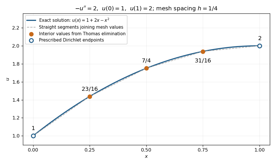
Exact quadratic Dirichlet Poisson solution and the three interior values recovered by tridiagonal elimination
. Details. For any interior points with , the scaled tridiagonal matrix has and . Its pivot elements are : start at and use . All are positive. Interior rows have equality in diagonal dominance, so strict diagonal dominance is not the reason this example works. Instead it is a symmetric positive-definite matrix, since for a real vector with ,Zero would force every neighbouring value equal and hence all values zero. This connects the boundary constraints directly to the safe pivots for tridiagonal elimination.
Let . Store the tridiagonal matrix by its diagonal , lower diagonal , and upper diagonal . The linear system iswith the nonexistent endpoint terms omitted. Initialize and . For , compute the elimination multiplier, modified pivot element, and modified right-hand side:These recurrence relations apply the elementary row operation after the preceding row has already been reduced. The transformed linear system is an upper bidiagonal matrix:Thus back substitution is especially short:For , only remains. Check each pivot element before its first division, including before back substitution.
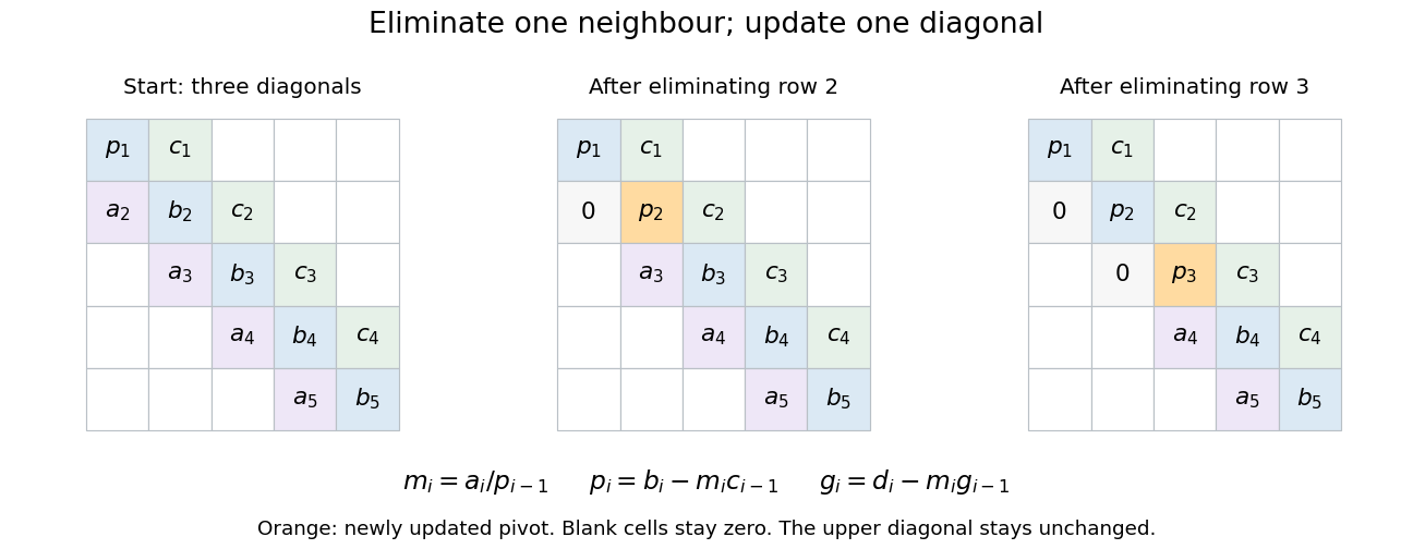
Tridiagonal elimination preserves the narrow band: only one row and one diagonal coefficient change per step
. Details. Equivalently, this constructs an LU decomposition with unit lower bidiagonal matrix , whose lower diagonal is , and upper bidiagonal matrix , whose diagonal is and upper diagonal is . The sweep is forward substitution in . There is no fill-in outside these bands when no rows are interchanged. LAPACK's
DGTSV source uses these same coefficient and right-hand-side updates in its branch without row interchange.[ref]A square triangular number is simultaneously a triangular number and a perfect square. For example, . This differs from a squared triangular number: is not itself triangular, by the recognition criterion for triangular numbers. Writing gives , a Pell equation that explains why this intersection of two counting patterns has additional arithmetic structure.
Pinned article: Introduction to the OurBigBook Project
Welcome to the OurBigBook Project! Our goal is to create the perfect publishing platform for STEM subjects, and get university-level students to write the best free STEM tutorials ever.
Everyone is welcome to create an account and play with the site: ourbigbook.com/go/register. We belive that students themselves can write amazing tutorials, but teachers are welcome too. You can write about anything you want, it doesn't have to be STEM or even educational. Silly test content is very welcome and you won't be penalized in any way. Just keep it legal!
Intro to OurBigBook
. Source. We have two killer features:
- topics: topics group articles by different users with the same title, e.g. here is the topic for the "Fundamental Theorem of Calculus" ourbigbook.com/go/topic/fundamental-theorem-of-calculusArticles of different users are sorted by upvote within each article page. This feature is a bit like:
- a Wikipedia where each user can have their own version of each article
- a Q&A website like Stack Overflow, where multiple people can give their views on a given topic, and the best ones are sorted by upvote. Except you don't need to wait for someone to ask first, and any topic goes, no matter how narrow or broad
This feature makes it possible for readers to find better explanations of any topic created by other writers. And it allows writers to create an explanation in a place that readers might actually find it.
Figure 1. Screenshot of the "Derivative" topic page. View it live at: ourbigbook.com/go/topic/derivativeVideo 2. OurBigBook Web topics demo. Source. - local editing: you can store all your personal knowledge base content locally in a plaintext markup format that can be edited locally and published either:This way you can be sure that even if OurBigBook.com were to go down one day (which we have no plans to do as it is quite cheap to host!), your content will still be perfectly readable as a static site.
- to OurBigBook.com to get awesome multi-user features like topics and likes
- as HTML files to a static website, which you can host yourself for free on many external providers like GitHub Pages, and remain in full control

Figure 2. You can publish local OurBigBook lightweight markup files to either OurBigBook.com or as a static website.
Figure 3. Visual Studio Code extension installation.
Figure 5. . You can also edit articles on the Web editor without installing anything locally. Video 3. Edit locally and publish demo. Source. This shows editing OurBigBook Markup and publishing it using the Visual Studio Code extension. 
- Infinitely deep tables of contents:




All our software is open source and hosted at: github.com/ourbigbook/ourbigbook
Further documentation can be found at: docs.ourbigbook.com
Feel free to reach our to us for any help or suggestions: docs.ourbigbook.com/#contact