Topics (384k) Articles (398k) Users (410) Discussions (242) Comments (383) Files (13k) New article

For an orthonormal wavelet and its scaling function, set and similarly for . The coarse scaling functions together with nonnegative-resolution wavelets form an orthonormal basis of . The coefficients are the corresponding L2 inner products. The series converges in the L2 norm, and the Parseval identity for a Hilbertian basis equates squared norm with the sum of squared coefficients. Pointwise convergence requires additional hypotheses.
A discrete wavelet transform computes multiscale approximation and detail coefficients from sampled data. For the Haar wavelet, replace each adjacent pair byThe approximation coefficient is times the pair's arithmetic mean; it is not the ordinary mean. The detail coefficient records their signed contrast. Repeat on the approximation coefficients until only one remains, keeping every detail coefficient.
For a worked example, start with the vector . The first pass gives approximation coefficients and detail coefficients . Transforming the remaining pair gives the coarse coefficient and the half-to-half detail . In the order coarse value, coarse detail, then fine details, the transform isThis is an orthogonal matrix transformation. Each pair preserves , so the full transform preserves the squared Euclidean norm:The inverse function for each pair is , . Reversing the passes therefore recovers every original value. This squared-norm bookkeeping is often called signal energy; it need not represent physical energy. [ref]
https://www.mathworks.com/help/wavelet/ug/haar-transforms-for-time-series-data-and-images.html. MathWorks: Haar transforms, approximation/detail coefficients and squared-norm conservation
Continuous and discrete normalizations differ. If data values are interpreted as the heights of a step function on equal cells of , its normalized L2 inner product coefficients are the discrete coefficients divided by . For our four values they are , as the Haar projection example shows. The same normalization is used by the wavelet regression estimator on .
Under independent Gaussian noise with a common variance, orthogonality preserves that coefficient noise variance and independence. It does not make every arbitrary correlated signal independent: this statistical conclusion uses the Gaussian model and its equal-variance independent inputs.
If a wave packet experiences a fractional nonlinear change per interaction, and successive interaction phases are decorrelated, changes add as a random walk of size . Order-one transfer needs interactions, giving the displayed cascade time. Phase coherence or resonant constraints can alter this estimate; weakness alone does not justify random addition.
For a complex random wave amplitude, this two-point expectation retains the coherent field and uses a complex conjugate on the second amplitude. It is not a normalized wave-field correlation coefficient. Subtracting gives the centered covariance function. At coincident points the uncentered wave-field correlation equals the mean wave intensity. Under second-order stationarity it depends only on the separation and has a spectral measure of a stationary random field. A deterministic field is included by taking a degenerate ensemble.
For constant wave speed , the whole-line Cauchy problemhas the unique classical solution, for and ,The first term evolves displacement released from rest; the second evolves initial velocity. The factor converts an integral of velocity over distance into displacement. On a finite string the formula applies before the backward characteristic curves reach an endpoint, or globally after an extension that enforces the boundary conditions. [ref]
For a completely smooth example, choose a bump function with compact support:where sets the half-width and sets the initial peak. ThenAt the two copies coincide, recovering peak . At , . At the pulses are separated, centred at , each of width and peak . Zero initial velocity forces equal left and right contributions; a purely right-moving initial profile instead requires . Thus “released from rest” and “launched to the right” describe different Cauchy data.
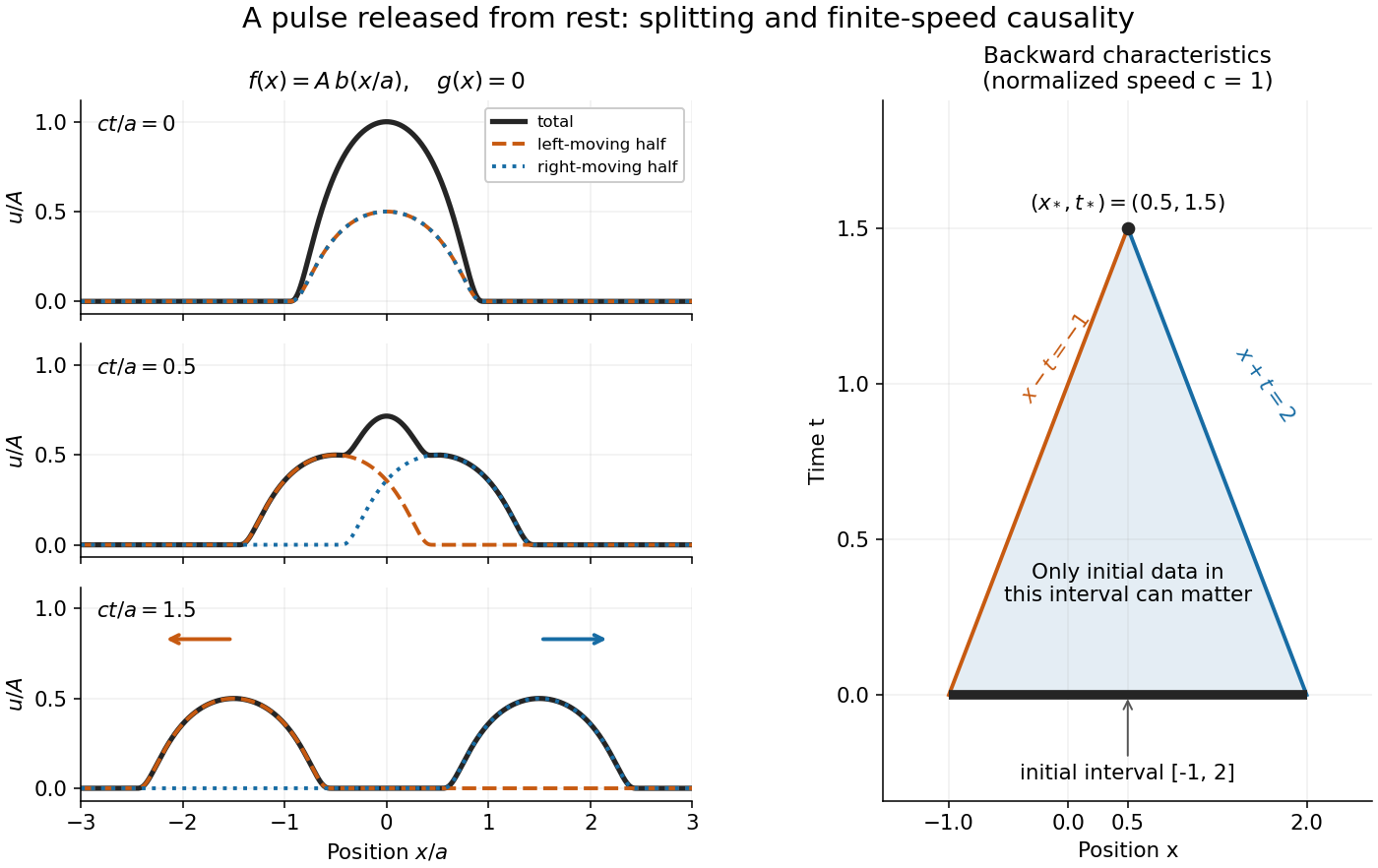
A smooth pulse released from rest splits in two, while backward characteristics select a causal interval
. Details. The domain of dependence of , for , is contained in on the initial line. More precisely, displacement contributes only through the two endpoints, while initial velocity contributes throughout the interval. With , and , that interval is . Changing either initial datum outside it cannot change . If both initial data vanish outside , the solution vanishes outside : this is finite propagation speed. The expanding interval bounds possible influence; it need not be filled by nonzero displacement, as the separated bumps demonstrate.
Historically, d'Alembert studied the vibrating-string problem in “Recherches sur la courbe que forme une corde tendue mise en vibration”, in the Berlin Academy's volume for the year 1747, pages 214–219. The memoir introduces the differential equation and integrates it through two arbitrary one-variable functions. The original geometric problem makes the formula's enduring appeal clear: arbitrary initial shapes can be handled without first decomposing them into normal modes. [ref]
https://webusers.imj-prg.fr/~david.aubin/cours/Textes/Dalembert-HAB-1747-cordes-vibrantes.pdf. D'Alembert, vibrating-string memoir, Academy year 1747
For a brief derivation, use characteristic coordinates and . The chain rule gives , so . The initial conditions yield and . Integrating these relations gives the displayed formula; the arbitrary integration constants cancel in their sum.
Damping dissipates the energy of an oscillation, reducing its amplitude. A linearly damped string applies this mechanism to each normal mode.
Why can stronger damping make a return to equilibrium slower? A weak brake lets a spring exchange potential energy with kinetic energy many times; a very strong brake makes the final motion creep. Critical damping marks the boundary between these behaviours. The distinction depends on the force law: the classification below concerns a single damped harmonic oscillator with viscous damping, rather than every mechanism that removes energy.
Let be displacement from equilibrium, the moving mass, the spring constant, and the constant coefficient of viscous damping. With no driving force, Newton's second law givesThe two initial conditions specify displacement and velocity. Define the undamped eigenfrequency as an angular frequency and the damping ratio as . The ordinary differential equation becomes . A constant weight in a vertical spring merely shifts equilibrium; it is already absorbed in the definition of .[ref]
For example, the ideal parameters and give and critical damping at . Values give damping ratios , respectively. These are model choices, not measured values. For release from rest with , set and ; then , where primes now denote derivatives with respect to .
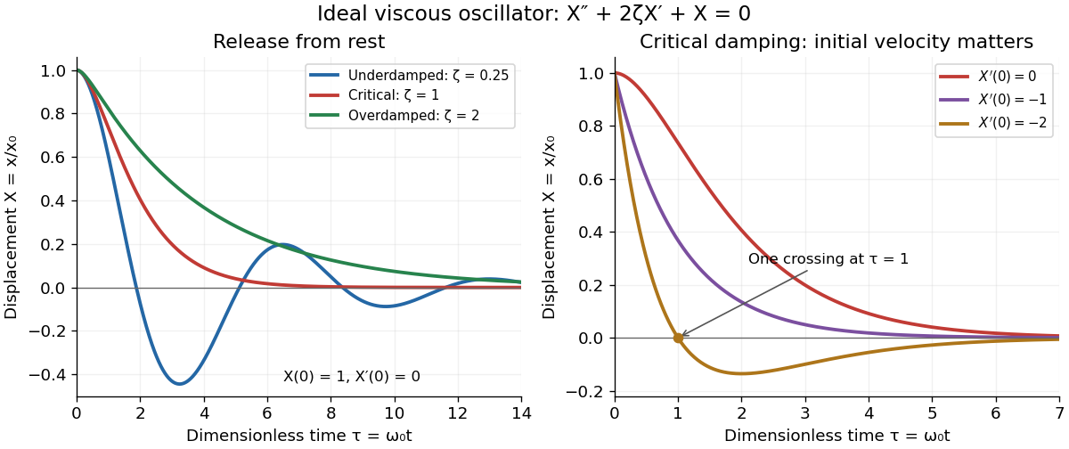
Ideal viscous oscillator responses: release from rest in three damping regimes, and the effect of initial velocity at critical damping
. Details. The left panel uses identical initial conditions , . Underdamping produces repeated crossings of equilibrium; critical damping and overdamping give positive decreasing responses. The right panel keeps critical damping but changes initial velocity: gives one crossing, although there is no oscillation. Both panels are exact model predictions.
For a spherically symmetric function, reduces the radial wave equation to . A time-harmonic separated solution has radial numerator , with . Finiteness at the origin excludes , and the prescribed finite origin value fixes . This is a standing combination of incoming and outgoing waves. A purely outgoing point-source wave instead has a singularity and must be specified by its source strength, not by a finite value at the origin.
For small quasi-geostrophic approximation waves on a locally uniform basic zonal flow with nonzero meridional potential-vorticity gradient , this signed quadratic wave activity obeys , where is the Eliassen–Palm flux and is a PV source. Multiply the linear PV equation by and use the Taylor identity for quasi-geostrophic flux to obtain it. In a locally uniform conservative wave packet, , so the flux follows the group velocity, with its sign determined by .
For a small-amplitude conservative wave packet in a slowly varying fluid flow, its intrinsic energy divided by intrinsic frequency is transported along its group velocity, with the basic advection added in the laboratory frame. A stationary background conserves laboratory angular frequency, but a changing mean velocity changes the intrinsic one through the Doppler effect; intrinsic energy alone need not be conserved. Geometrical spreading and dissipation enter the action-flux balance.
The moments of the mutation count on a neutral coalescent tree give this variance for . Since and the sum of inverse squares is bounded, it tends to zero. Together with unbiasedness, this gives mean-square convergence to the mutation parameter, so it is a consistent estimator.
For fixed , a geometric mutation count in a coalescent epoch with mean has third moment . The centered absolute third moment is at most , so its sum is . The total variance is asymptotic to , making the Lyapunov condition with hold. Rescaling by the harmonic sum gives the displayed limit. At the estimator is identically zero and the limit is degenerate. The variance of the Watterson estimator decreases only logarithmically with sample size at a fixed nonrecombining locus.
The local skin friction coefficient normalizes wall shear stress by the outer dynamic pressure:For the ideal Blasius boundary layer on one face of length , averaging the local skin friction coefficient gives . The factor of two follows from integrating , not from counting both plate faces. Drag on two equally exposed faces doubles when the reference area remains that of one face.
A trail is a walk whose edge sequence has no repetitions. Its vertices may repeat, including its first and last vertices. The zero-length walk is a trail because it repeats no edge. Every graph path is a trail, but the converse fails: the trail in the shared example isIts six edges are pairwise distinct, although occurs twice. Visiting a junction again and traversing a road segment again are different events.[ref]
https://people.math.binghamton.edu/zaslav/Oldcourses/581.S99/notes.html. Thomas Zaslavsky, Supplementary Notes for Graduate Graph Theory: trails and paths
In an undirected graph, traversing and then repeats the same edge; direction of travel does not give it a new identity. In a multigraph with distinct parallel edges joining and , the closed walk is a trail, whereas is not. Both have the same vertex sequence . In a directed graph, separate directed edges and may instead be used once each; record their identities and obey their directions. Thus testing a trail means checking the actual edge records, not merely checking consecutive endpoint labels.
For a finite graph, a trail has length at most ; unrestricted walks can have arbitrarily large length whenever a positive-length closed walk exists, since it can be repeated. An Eulerian trail is the special trail that uses every edge, so its length is exactly . Our length-six trail omits and is therefore not an Eulerian trail. In a road-inspection model, a trail describes servicing its selected segments once while allowing returns to junctions; requiring service of every segment leads to the Eulerian trail question. If extra travel between serviced segments is necessary, the complete journey can be a walk even when each segment is serviced only once. This distinction keeps the service requirement separate from the route actually travelled.
For a simple symmetric random walk starting at zero, let be its first hitting time of . The infinite mean first passage of a simple symmetric random walk shows that almost surely but . Since , assuming a finite expected value for would let Wald's equation assert , a contradiction. The formal expression is not an allowed use of the theorem.[ref]
Compare . From every surviving position in , three consecutive positive increments force absorption within three steps. Each fresh block has probability of this event, so and . This establishes finiteness before invoking the theorem. If is the average remaining time from position , the law of total expectation givesso . Symmetry gives equal exit probabilities at and , and , as Wald's equation predicts. This is a small gambler's ruin problem with two absorbing barriers.
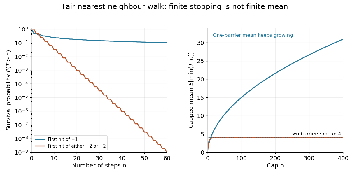
Even for , each bounded stopping time satisfies . The stopped process tends to almost surely, but its expected value does not tend to . Rare long negative excursions retain the balancing contribution. The existing stopped-walk martingale with almost sure but not L1 convergence explains the related failure of uniform integrability; almost sure convergence alone does not permit exchanging a limit and an expected value.
Let be independent fair signs, each taking and with equal probability. Set if , and if . Deciding whether requires the second sign, so is not a stopping time for the natural filtration. The four equally likely possibilities giveBoth the increments and the count are bounded, but the identity fails because the second contribution is retained only when it is negative. This is selection using an unobserved outcome, rather than a legitimate sequential decision. Boundedness alone cannot replace the stopping time hypothesis.[ref]
Consider a stipulated repeated-attempt model, with independent Bernoulli trials of success probability . An unsuccessful attempt costs three units of work, and a successful attempt costs one. Let be its success indicator function, its cost, and the first success. Observing reveals , so is a stopping time for the costs' natural filtration. The geometric distribution gives and , including the deterministic case . ThusAt , the average is four attempts and ten units of work. An independent check uses the pathwise identity : there are failures and one final success. No success probabilities or costs in this example are measured data.
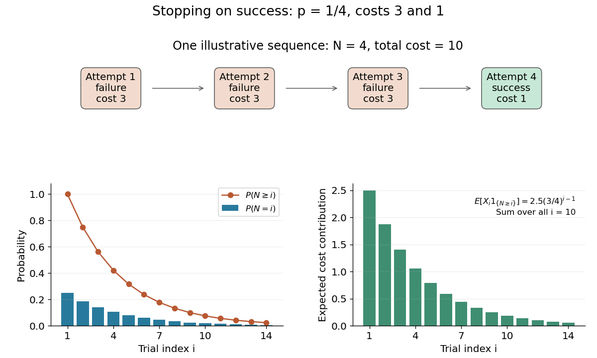
Cost and survival probabilities for stopping at the first success
. Original stipulated model with success probability , failure cost three, and success cost one. The top shows one illustrative stopped sequence; the lower panels show exact probabilities and the contributions to the expected value from each admitted step. Details.Here is not independent of the observed costs. In particular, conditioning on forces every preceding cost to be three and the final cost to be one, so , generally different from at . Nevertheless the unconditional identity holds. This distinction explains why conditioning on the total count as though the original cost law remained unchanged is a faulty proof.
An ideal straight line vortex in a two-dimensional incompressible flow has circulation and induces velocityIts stream function, with , is . Positive means counterclockwise circulation. In an ideal point-vortex description, the vortex position is advected by the regular velocity produced by the other vortices and the boundaries; its own singular velocity is excluded.
The evolution of a vorticity distribution together with the velocity field it induces. A transport equation advances vorticity; diagnostic inversion recovers velocity from it and the specified boundary conditions.
For density operators supported on mutually orthogonal subspaces, the eigenvalues of their mixture are , where are the eigenvalues of . Substitution into the definition of Von Neumann entropy gives the displayed decomposition into Shannon entropy of the label and the mean entropy within each block. Zero eigenvalues use .
Pinned article: Introduction to the OurBigBook Project
Welcome to the OurBigBook Project! Our goal is to create the perfect publishing platform for STEM subjects, and get university-level students to write the best free STEM tutorials ever.
Everyone is welcome to create an account and play with the site: ourbigbook.com/go/register. We belive that students themselves can write amazing tutorials, but teachers are welcome too. You can write about anything you want, it doesn't have to be STEM or even educational. Silly test content is very welcome and you won't be penalized in any way. Just keep it legal!
Intro to OurBigBook
. Source. We have two killer features:
- topics: topics group articles by different users with the same title, e.g. here is the topic for the "Fundamental Theorem of Calculus" ourbigbook.com/go/topic/fundamental-theorem-of-calculusArticles of different users are sorted by upvote within each article page. This feature is a bit like:
- a Wikipedia where each user can have their own version of each article
- a Q&A website like Stack Overflow, where multiple people can give their views on a given topic, and the best ones are sorted by upvote. Except you don't need to wait for someone to ask first, and any topic goes, no matter how narrow or broad
This feature makes it possible for readers to find better explanations of any topic created by other writers. And it allows writers to create an explanation in a place that readers might actually find it.
Figure 1. Screenshot of the "Derivative" topic page. View it live at: ourbigbook.com/go/topic/derivativeVideo 2. OurBigBook Web topics demo. Source. - local editing: you can store all your personal knowledge base content locally in a plaintext markup format that can be edited locally and published either:This way you can be sure that even if OurBigBook.com were to go down one day (which we have no plans to do as it is quite cheap to host!), your content will still be perfectly readable as a static site.
- to OurBigBook.com to get awesome multi-user features like topics and likes
- as HTML files to a static website, which you can host yourself for free on many external providers like GitHub Pages, and remain in full control

Figure 2. You can publish local OurBigBook lightweight markup files to either OurBigBook.com or as a static website.
Figure 3. Visual Studio Code extension installation.
Figure 5. . You can also edit articles on the Web editor without installing anything locally. Video 3. Edit locally and publish demo. Source. This shows editing OurBigBook Markup and publishing it using the Visual Studio Code extension. 
- Infinitely deep tables of contents:




All our software is open source and hosted at: github.com/ourbigbook/ourbigbook
Further documentation can be found at: docs.ourbigbook.com
Feel free to reach our to us for any help or suggestions: docs.ourbigbook.com/#contact