Topics (384k) Articles (398k) Users (410) Discussions (242) Comments (383) Files (13k) New article

The local meridional eddy buoyancy flux is the covariance of disturbance meridional velocity with disturbance buoyancy. In a Boussinesq approximation, . This is a local transport density, distinct from a plume's cross-section-integrated buoyancy flux. In the transformed Eulerian mean, division by the background buoyancy frequency squared gives an eddy-induced meridional overturning streamfunction.
A statistic is invariant if ; it is maximal when it also separates different group orbits. Consequently every invariant procedure factors through the maximal invariant, subject to the usual measurability conditions on the orbit space. Standardizing a sample by an equivariant estimator of location and positive scale gives a maximal invariant for the positive affine group.
An estimator respects the group action if the displayed identity holds. If it takes values in the transformation group itself, normalization is a maximal invariant: equivariance proves invariance, and equality of normalized samples reconstructs the transformation between them. For estimates in a homogeneous parameter space with a nontrivial stabilizer, normalization is defined only modulo that stabilizer; quotienting the remaining action is essential.
Hubbard-Stratonovich decoupling of an exponentially coupled Ising chain gives a scalar-field action with a nearest-neighbor gradient term and . Its continuum partition function is the Euclidean path integral of the displayed quantum particle. At zero field the potential can have two wells, but a finite barrier still permits quantum tunnelling and gives a unique symmetric ground state. The excitation gap produces a finite classical correlation length, so there is no finite-temperature spontaneous magnetization for fixed positive . One classical spatial coordinate becomes imaginary time; a -dimensional classical model corresponds to a quantum model with spatial dimensions.
The hypothesis makes abelian and makes any two conjugate elements of equal. For the latter assertion, Sylow conjugacy inside the centralizer of the target element adjusts a conjugating element into , where it centralizes . Evaluating group transfer to on an element , each coset cycle contributes a conjugate of raised to the cycle length, hence that same power of . The restriction is consequently , an automorphism of the abelian -group. Transfer is surjective, and its kernel is the required normal p-complement.
For a specified transcription unit, the coding strand is the DNA strand matching the initial RNA product in the direction, with T in place of U. The opposite DNA strand is the template. The name does not imply that every transcribed gene encodes a protein. See Clark, Douglas and Choi: coding and template strands.
An RNA polymerase used in transcription is an enzyme that synthesizes RNA from a DNA template. Unlike a replicating DNA polymerase, it can start a new strand without a pre-existing paired strand end; initiation still requires the appropriate DNA signals and associated machinery. See Alberts et al.: RNA polymerase and transcription initiation.
For distinct algebraic numbers , the numbers are linearly independent over . Equivalently, exponentials of numbers linearly independent over are algebraically independent over . The special case of a nonzero algebraic exponent gives a transcendental exponential. In particular forces to be transcendental.
In the modern strict sense an E-function satisfies a nonzero linear differential equation over , has algebraic coefficients with all conjugates bounded by , and has common positive denominators making algebraic integers. Siegel's original arithmetic growth condition permits, for each , bounds of size instead. The strict and original growth formulations should be distinguished rather than asserted equivalent. Exponentials with algebraic exponent satisfy the stronger conditions and a first-order differential equation.
Mahler's method uses functional equations relating a function at and at to transport an auxiliary polynomial to points rapidly approaching zero. High vanishing order gives an upper bound which conflicts with an algebraic norm or height lower bound under assumed algebraicity of the values. Functional transcendence ensures that the auxiliary expression is not identically zero.
For algebraic and algebraic irrational , every value with is transcendental. Consequently any quotient of chosen nonzero logarithms of algebraic numbers is either rational or transcendental.
Suppose nonzero algebraic numbers form a Galois-stable set, with Galois-invariant integer weights , and is an integer. Choose vanishing at all with , and a positive integer making all algebraic integers. For a large prime , put and , and let be the sum of its derivatives. The weighted sum is an integer, nonzero modulo when . If the displayed exponential expression vanished, integrating along the finitely many segments to would bound that nonzero integer by . This contradiction proves the obstruction and supplies direct proofs for and .
Let be meromorphic functions with for a fixed number field . Suppose are algebraically independent over and have finite orders . The set of points where every is finite and belongs to satisfies the displayed bound. The orders are growth orders for meromorphic functions. For , , the orders are zero and one and the functions are algebraically independent; an algebraic value of at nonzero algebraic would produce infinitely many such points .
The steady-state tracking error iswhen this finite limit exists. A finite steady-state tracking error does not require the reference signal, the plant output, or the control input to become constant: all can grow while their difference settles. If the tracking error grows without bound or keeps oscillating, report that behavior rather than assigning a finite steady-state tracking error. Eventual accuracy and asymptotic stability are different questions.
For the first-order low-pass filter introduced in reference signal, assume exact measurement, constant control disturbance , and no actuator saturation or feedback delay. Under proportional control with , a constant reference signal givesThe decaying homogeneous solution has rate , so this equilibrium point is approached from any finite initial condition. A nonzero tracking error is needed to maintain the control input that balances the model's tendency to relax toward . This differs from the accumulating controlled plant , for which proportional control already tracks a constant reference signal exactly when . The presence or absence of a step offset depends on both the controlled plant and the controller.
For a ramp reference signal , the same proportional control givesIts long-time particular solution grows with slope when . Thus the controlled plant and homogeneous closed-loop response are stable, but the tracking error has no finite steady-state tracking error. A changing goal requires a different performance test from a fixed destination.
Now use proportional-integral control , , with . For the same controlled plant, differentiate the error equation on intervals where the inputs are smooth:The characteristic polynomial has both roots of a polynomial in the open left half-plane: real roots have negative sum and positive product, and a nonreal complex conjugate pair has negative real part. This proves decay of the homogeneous error for this model. It does not prove stability of an arbitrary controlled plant controlled by positive gains. At a reference jump, use the original ordinary differential equations to set the new initial conditions, rather than treating the reference as smooth at that jump.
With a constant reference signal and constant control disturbance, proportional-integral control therefore gives . At its equilibrium point, , , and . The stored integral maintains the required command while the current tracking error vanishes. For a ramp reference signal, however, the forcing above is , andThe tracking error settles even though the accumulated integral and the required control input grow. This finite offset is the error needed to keep increasing that command. For with , the forcing is and even this proportional-integral control leaves a tracking error growing with slope . Integral action is therefore a precise mechanism for selected input classes, not a promise of perfect tracking for every reference signal. [ref]
https://www.fbswiki.org/wiki/index.php/PID_Control. Åström and Murray, Feedback Systems, Chapter 11: integral action and actuator limits
Here are completely explicit synthetic examples with , , and no sensor bias. Choose , per percentage point, percentage point per degree, and percentage points per degree-second. Thus is dimensionless, and . In the following formulas, denotes the numerical time in seconds and denote numerical temperature rises in degrees. For the unit-step reference signal , proportional control and proportional-integral control respectively giveFor the ramp reference signal , the corresponding solutions areThe control inputs here are numerical heater-command percentage points. Substitution into and into the controller equations checks these solutions without invoking an unverified limiting rule. The proportional control step offset is degrees; the proportional-integral control step offset is zero. The proportional control ramp error grows; the proportional-integral control ramp offset is degrees, exactly .
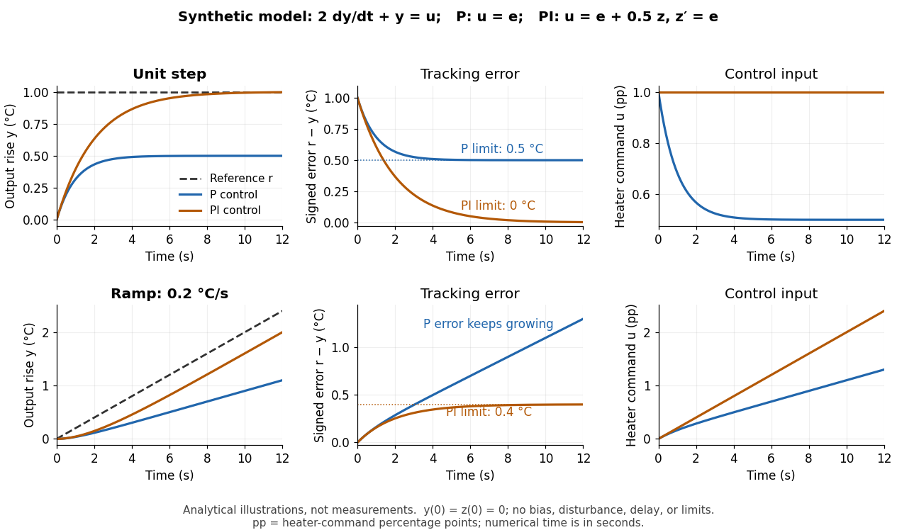
Synthetic step and ramp tracking of one stable first-order low-pass filter
. Original analytical model curves, not measurements or fits to the temperature laboratory. Columns compare plant output with reference signal, signed tracking error, and control input; rows use a unit step and a ramp of degrees per second. Both designs have decaying homogeneous responses. Proportional-integral control removes the step offset but leaves the ramp offset degrees; proportional control has an increasing ramp error. Heater-command percentage points and output degrees use separate axes. Details.The conclusions have specific limits. With constant sensor bias , stable proportional-integral control for a feasible constant reference signal drives the measured tracking error to zero but leaves the physical discrepancy . Under proportional control, the measured offset instead becomes . If actuator saturation prevents the required control input, zero step offset is not achievable by these formulas. A changing control disturbance contributes to the error equation, while feedback delay can change stability; neither is covered by the constant-disturbance result. These restrictions are what make steady-state tracking error useful: it identifies the input, measurement convention, and model for which an accuracy claim is actually justified.
For two normalized pure states, the difference of their projectors has two eigenvalues , giving that trace distance. Write a mixed density operator as . Convexity of the trace norm and weighted Cauchy-Schwarz inequality give . Thus a small probability of failing the pure-state projector test forces trace-distance proximity, including for correlated multipartite outputs.
For the pure qubit , subtracting the output of dephasing channel leaves a Hermitian matrix with zero diagonal and off-diagonal modulus . Its two eigenvalues are that number and its negative, giving the displayed trace distance. For real , this is .
By the variational characterization of trace distance, maximize over . The adjoint of a quantum channel is positive and unital, so . Moving the channel onto therefore restricts, rather than enlarges, the effects available in the input variational problem. This proves the displayed bound for every pair of density operators.
For qubit density operators, the trace distance has a particularly simple geometry. Write their Bloch vectors as in the Bloch ball:where is the identity operator and denotes the Pauli matrices. This Bloch vector representation includes both pure states on the Bloch sphere and mixed states in the interior of the Bloch ball. [ref]
The Pauli matrix multiplication law gives . Hence the two eigenvalues of are , and their absolute sum givesThe trace distance is half the straight-line Euclidean distance between the Bloch vectors, not the angular or surface distance along the Bloch sphere. Opposite Bloch vectors have trace distance one; the centre is at trace distance from every pure state.
For the pure states and , the Bloch vectors are and . Their straight-line separation is , soThese Bloch vectors are perpendicular, but the pure states are not orthogonal: . The Helstrom measurement for the zero and plus states measures along the difference direction , rather than along either input Bloch vector.
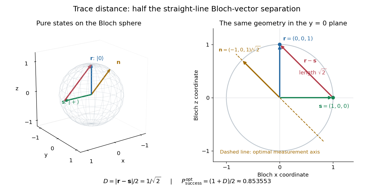
Trace distance is half a Bloch-vector chord, and the optimal zero-versus-plus measurement follows the difference direction
. Details. Count the ancestor and the next generations of a Galton-Watson process. Conditioning on the ancestor's offspring, their independent descendant trees each have the preceding finite-horizon probability generating function, proving the displayed recursion. If the count instead excludes the ancestor, the recursion is with . The indexing convention must be specified.
The abstract of Information Theoretical Analysis of Multivariate Correlation by Satosi Watanabe (1960, printed p. 66) names the sum of individual information entropies minus joint entropy "total correlation." It presents this as the finest grouping of the variables and identifies applications to geometric pattern recognition and shuffling cards marked zero or one. The name therefore connects the uncertainty of a system with the structure linking its parts; the worked integer parity and noisy-integer parity models here are separate examples calculated from their stated laws.
Pinned article: Introduction to the OurBigBook Project
Welcome to the OurBigBook Project! Our goal is to create the perfect publishing platform for STEM subjects, and get university-level students to write the best free STEM tutorials ever.
Everyone is welcome to create an account and play with the site: ourbigbook.com/go/register. We belive that students themselves can write amazing tutorials, but teachers are welcome too. You can write about anything you want, it doesn't have to be STEM or even educational. Silly test content is very welcome and you won't be penalized in any way. Just keep it legal!
Intro to OurBigBook
. Source. We have two killer features:
- topics: topics group articles by different users with the same title, e.g. here is the topic for the "Fundamental Theorem of Calculus" ourbigbook.com/go/topic/fundamental-theorem-of-calculusArticles of different users are sorted by upvote within each article page. This feature is a bit like:
- a Wikipedia where each user can have their own version of each article
- a Q&A website like Stack Overflow, where multiple people can give their views on a given topic, and the best ones are sorted by upvote. Except you don't need to wait for someone to ask first, and any topic goes, no matter how narrow or broad
This feature makes it possible for readers to find better explanations of any topic created by other writers. And it allows writers to create an explanation in a place that readers might actually find it.
Figure 1. Screenshot of the "Derivative" topic page. View it live at: ourbigbook.com/go/topic/derivativeVideo 2. OurBigBook Web topics demo. Source. - local editing: you can store all your personal knowledge base content locally in a plaintext markup format that can be edited locally and published either:This way you can be sure that even if OurBigBook.com were to go down one day (which we have no plans to do as it is quite cheap to host!), your content will still be perfectly readable as a static site.
- to OurBigBook.com to get awesome multi-user features like topics and likes
- as HTML files to a static website, which you can host yourself for free on many external providers like GitHub Pages, and remain in full control

Figure 2. You can publish local OurBigBook lightweight markup files to either OurBigBook.com or as a static website.
Figure 3. Visual Studio Code extension installation.
Figure 5. . You can also edit articles on the Web editor without installing anything locally. Video 3. Edit locally and publish demo. Source. This shows editing OurBigBook Markup and publishing it using the Visual Studio Code extension. 
- Infinitely deep tables of contents:




All our software is open source and hosted at: github.com/ourbigbook/ourbigbook
Further documentation can be found at: docs.ourbigbook.com
Feel free to reach our to us for any help or suggestions: docs.ourbigbook.com/#contact