Topics (384k) Articles (398k) Users (410) Discussions (242) Comments (383) Files (13k) New article

For initial asset value , final value , and intervening cash distribution , the net financial return is . Its gross return is . In a one-period portfolio with initial-value weights summing to one, the net return is . The expected return is its expected value; a realized return need not equal it.
The incubation period is the interval from infection to symptom onset in a person who develops symptoms. Its probability distribution describes onset times, not the full timing of infectiousness. Exposure may only be known to fall in an interval, requiring a corresponding observation model when estimating this distribution.
Quarantine restricts contacts of exposed individuals whose infection status is uncertain, with monitoring to detect illness. It differs from isolation of recognized infected or ill individuals. An incubation period quantile can enter a duration calculation, but assumptions about exposure time, symptom detection and infectiousness are needed before the calculation describes transmission risk.
In a continuous-time epidemic model, a constant recovery rate gives an exponential distribution of infectious duration with mean . Other duration distributions require additional stages or infection-age structure.
A stochastic epidemic model represents infection and recovery as random events. A continuous-time Markov chain can track integer counts, while a stochastic SIR model illustrates random fade-out and finite-population outbreak variability that a deterministic limit does not show.
A macroparasite burden model tracks the distribution of within-host parasite burdens and couples it to transmission or environmental infectious stages. Mean burden alone is insufficient when worm mating, nonlinear fecundity, immunity or host mortality depend on that distribution.
Each undirected cross-group partnership is counted once from each group's contact total. Thus group size times per-person contact rate times cross-group fraction must agree. If one group occupies fraction while its cross-group per-person rate stays fixed, aggregate cross-group contact is order and the other group's cross-contact fraction is order . Assigning both per-person rates independently generally breaks this balance.
For a smoothly moving volume whose boundary has normal velocity , the derivative of an integral equals the local time-change integral plus the boundary-transport flux. The boundary term comes from the thin layer swept by the moving surface during a short time interval. Taking gives . If the boundary moves with the fluid, this combines with the divergence theorem to give the integral of the material derivative plus times the velocity divergence.
The magnetic helicity integrates the dot product of a magnetic vector potential and its magnetic field. It measures linkage and twisting of magnetic flux. For a solenoidal vector field tangent to the boundary, it is unchanged by the gauge transformation , since the change is . If its density satisfies with both vector fields tangent to the boundary of a fixed volume, the divergence theorem gives conservation of its integral. This is an instance of helicity conservation by tangent boundary conditions.
A Gouy balance detects the force exerted by a nonuniform magnetic field on a sample of uniform cross-section extending between high- and low-field regions. TeachSpin's implementation reverses the usual arrangement: a rare-earth permanent-magnet assembly sits on a one-pan electronic balance, while a separate holder brings the sample into the field. The magnet's apparent mass change measures the opposite of the sample's vertical force, by Newton's third law. The described pole faces have diameter and separation ; samples occupy cuvettes of cross-section and height about . [ref]
Foundational Magnetic Susceptibility by TeachSpin. TeachSpin, Foundational Magnetic Susceptibility, Instrument: The Gouy Method and “Weighing the magnet” method; Specifications: magnet and sample dimensions
The same balance calibrates magnetic flux density by measuring the reaction force on the magnet when a wire of known horizontal length carries known electric current perpendicular to the field: . The manufacturer describes water being repelled by the high-field region, identifying negative magnetic susceptibility. This observed sign supplies a qualitative test, not a measured Curie's law curve. [ref]
Foundational Magnetic Susceptibility by TeachSpin. TeachSpin, Foundational Magnetic Susceptibility, Instrument: Absolute calibration method and Diamagnetism
For weak reversible linear response, a uniform sample displacing a weakly magnetic surrounding medium has, to leading order, downward forceThis follows by integrating the induced-dipole force density along a downward coordinate. is the cross-sectional area, and the two values are applied magnetic flux densities. The force depends on the endpoint fields; the entire field-gradient profile need not be measured under these assumptions. In the reversed apparatus, after subtracting the holder background, where is gravitational acceleration. This sign must be reversed before inferring volume magnetic susceptibility.
Useful controls are an empty-holder reading at the same position, a distant-sample baseline, repeated wire-current reversals during field calibration, and stable temperature. They separate holder response, balance drift, force offsets, and thermal changes; these are proposed checks for the stated inference. Finite endpoint fields, nonuniform cross-section, uneven powder packing, stray forces and a demagnetizing field limit the simple formula. If magnetization is nonlinear, the weak-response force involves instead of a constant- endpoint square. A balance reading then measures an integrated response, not directly the local differential magnetic susceptibility.
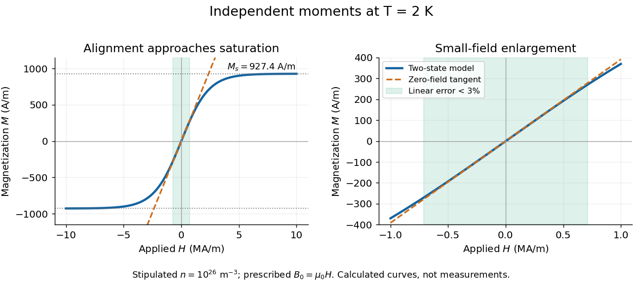
Saturation magnetization is the limiting magnetization when the responding magnetic moments are fully aligned within the stated model or experimental regime. In independent-moment magnetic response, . Reaching a large magnetization does not imply a large differential magnetic susceptibility: the remaining slope can be almost zero.
Consider a stipulated dilute collection of independent two-level systems, each with longitudinal magnetic moment , , and energy . The prescribed vacuum/applied magnetic flux density is . Ignore interactions, orbital magnetic response, and the small sample-field correction. This is the magnetic version of the existing independent spin-one-half two-level system, with alignment probabilities rather than an interacting Curie–Weiss model.
For temperature , the canonical ensemble gives the one-moment partition function , with . Taking the expected value over its two Boltzmann weights givesHere is the number density, the Boltzmann constant, and the hyperbolic tangent. For , its small-argument expansion of the hyperbolic tangent gives , a Curie's law response in the applied- convention. For large , approaches the saturation magnetization with sign set by the field, and its differential magnetic susceptibility falls towards zero.
Both plots use stipulated , , , and . The moment is approximately one Bohr magneton; the chosen vacuum permeability is a rounded model input. At , and . The linear approximation overestimates by less than for , corresponding to or . These parameters keep the modeled response weak; neglected magnetic feedback is of relative order , rather than an explanation of a material's ordered phase.
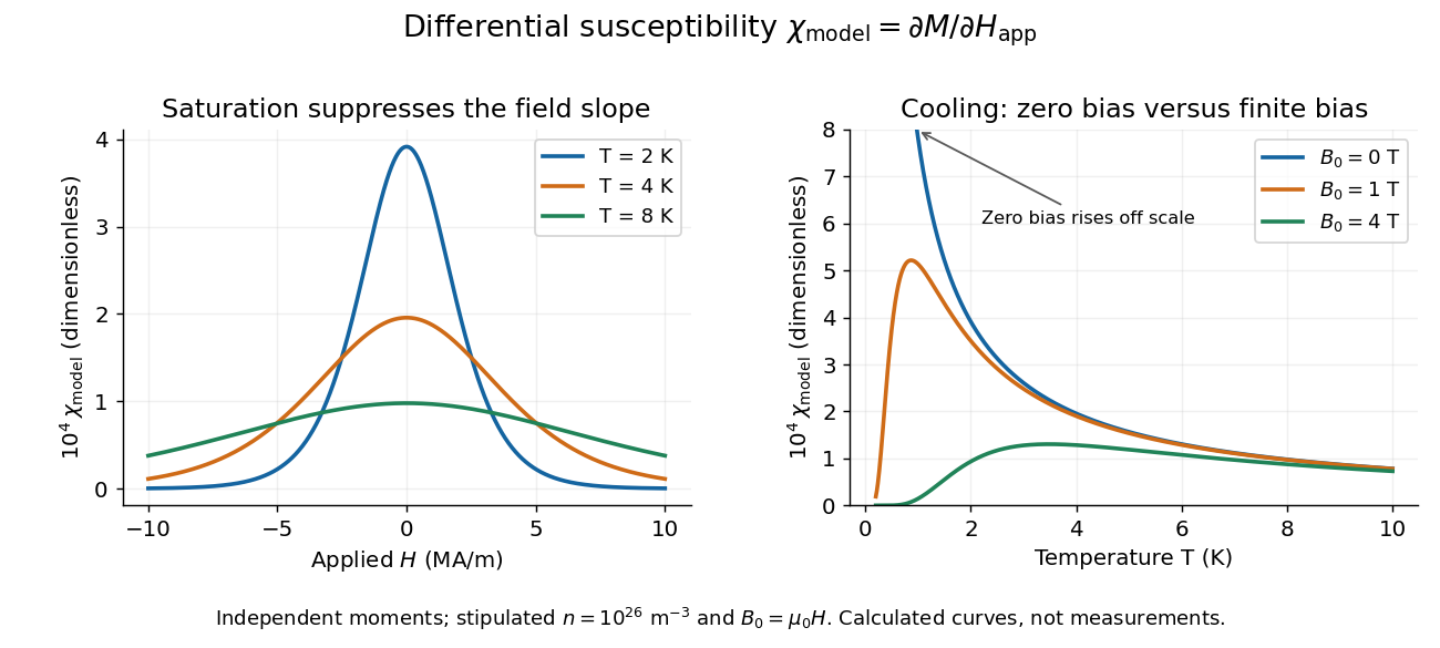
Bias-field and temperature dependence of the independent-moment differential magnetic susceptibility
. Original calculation using the same stipulated moments and number density. The left panel compares field sweeps at , and . The right panel compares temperature sweeps at prescribed , and . The zero-field slope follows Curie's law; cooling at fixed nonzero field eventually suppresses the slope through saturation magnetization. Details.At , cooling increases the zero-field slope as . At fixed , cooling instead gives : a saturated moment can hardly change further. The order of the zero-field and zero-temperature limits matters. This independent model has no finite-temperature collective phase transition; the diverging zero-field slope alone does not establish one.
The demagnetizing field is the contribution to magnetic field intensity produced by the sample's own magnetization. Inside a uniformly magnetized ellipsoid, it is uniform and has the form ; the demagnetizing factor along a principal axis gives its longitudinal component. These conditions make the scalar correction in field conventions for magnetic susceptibility useful.
A cylinder generally has spatially varying magnetization and demagnetizing field. A volume-sensitive instrument and a short central pickup coil consequently need different effective corrections: one averages over the sample, while the other samples central flux. A shape factor copied from an ellipsoid is not an exact correction for every cylinder, especially with nonlinear response or hysteresis. [ref]
Demagnetizing Factors. R. B. Goldfarb, Demagnetizing Factors, printed p. 104, §2 opening paragraphs: magnetometric versus fluxmetric sensing, nonuniform cylindrical fields and susceptibility-dependent factors
In vacuum, magnetization is zero and magnetic flux density obeys . The applied quantities and mean the field of the external sources at the sample position with the sample absent. The internal magnetic field intensity includes the sample's demagnetizing field; its internal magnetic flux density additionally includes . A field quoted in the tesla is a quantity, even when an instrument informally calls it “”.
For a uniformly magnetized ellipsoid, along a principal axis with demagnetizing factor in the International System of Units,For a sphere, . The axial value approaches zero in the long slender ellipsoid limit and the normal value approaches one in the thin flat ellipsoid limit. Thus a stipulated intrinsic volume magnetic susceptibility would yield apparent values in a sphere and approximately in a long axial sample. These are calculated geometry effects, not measured material values. For fixed , implicit differentiation gives the same conversion for local differential magnetic susceptibility, .
A magnetic susceptibility tensor maps a small change of internal magnetic field intensity to a change of magnetization:This tensor reduces to for isotropy. With anisotropy, even a linear response need not point along the applied magnetic field intensity. As a stipulated example, sends to . State the axes and bias field when reporting its components. A constant tensor describes linear response; in a nonlinear material it is the Jacobian matrix of the response at the chosen operating point.
Differential magnetic susceptibility is the local slope at a specified bias magnetic field intensity, holding temperature and other stated constraints fixed. It equals volume magnetic susceptibility only for a linear response through the origin. For example, has , but , where . At these are about and times their common zero-field slope. A finite sweep chord is another quantity, not automatically this derivative.
If the differentiated field is instead the internal magnetic flux density, the longitudinal chain rule applied to givesThis differs from the vacuum/applied- conversion in volume magnetic susceptibility. It assumes a differentiable single branch with locally invertible .
Volume magnetic susceptibility is the dimensionless ratio of longitudinal magnetization to internal magnetic field intensity in a linear regime through the origin. Positive response gives paramagnetism. Always distinguish magnetization from total magnetic moment : dividing by volume changes the normalization. Mass-normalized and mole-normalized values likewise require the mass density or the volume per amount of substance before comparison with .
In the existing Pauli paramagnetism formula, denotes total magnetic moment, and is the total spin-summed density of states. Relabel that response asHere is the Bohr magneton. If its is a prescribed vacuum/applied magnetic flux density , the dimensionless apparent slope is . It agrees approximately with intrinsic only when the demagnetizing field correction and magnetic feedback are negligible. The existing Curie's law formula also uses a total-magnetic moment, -derivative convention; its counts moments rather than giving a number density.
Curie's law is the inverse-temperature magnetic response of independent magnetic moments in the weak-polarization regime. Let each moment have angular momentum quantum number , Landé g-factor , and magnetic projection , where . Its Zeeman energy is . At zero field the projections are equally likely, so and . Differentiating their canonical partition function gives the total-moment response of independent moments,For a dilute weakly magnetized sample with number density and , the dimensionless SI volume magnetic susceptibility is insteadThese conventions differ by volume, field and factors. A fixed nonzero field eventually saturates the moments as temperature falls, so the linear Curie's law regime requires .[ref]
3 Quantum Gases. magnetic response and Curie's law; Tong defines susceptibility using total moment differentiated with respect to B
The London equations relate the superconducting electric current to the electromagnetic field: and . In a gauge with constant condensate phase the second follows from ; it implies exponential magnetic field screening.
Pinned article: Introduction to the OurBigBook Project
Welcome to the OurBigBook Project! Our goal is to create the perfect publishing platform for STEM subjects, and get university-level students to write the best free STEM tutorials ever.
Everyone is welcome to create an account and play with the site: ourbigbook.com/go/register. We belive that students themselves can write amazing tutorials, but teachers are welcome too. You can write about anything you want, it doesn't have to be STEM or even educational. Silly test content is very welcome and you won't be penalized in any way. Just keep it legal!
Intro to OurBigBook
. Source. We have two killer features:
- topics: topics group articles by different users with the same title, e.g. here is the topic for the "Fundamental Theorem of Calculus" ourbigbook.com/go/topic/fundamental-theorem-of-calculusArticles of different users are sorted by upvote within each article page. This feature is a bit like:
- a Wikipedia where each user can have their own version of each article
- a Q&A website like Stack Overflow, where multiple people can give their views on a given topic, and the best ones are sorted by upvote. Except you don't need to wait for someone to ask first, and any topic goes, no matter how narrow or broad
This feature makes it possible for readers to find better explanations of any topic created by other writers. And it allows writers to create an explanation in a place that readers might actually find it.
Figure 1. Screenshot of the "Derivative" topic page. View it live at: ourbigbook.com/go/topic/derivativeVideo 2. OurBigBook Web topics demo. Source. - local editing: you can store all your personal knowledge base content locally in a plaintext markup format that can be edited locally and published either:This way you can be sure that even if OurBigBook.com were to go down one day (which we have no plans to do as it is quite cheap to host!), your content will still be perfectly readable as a static site.
- to OurBigBook.com to get awesome multi-user features like topics and likes
- as HTML files to a static website, which you can host yourself for free on many external providers like GitHub Pages, and remain in full control

Figure 2. You can publish local OurBigBook lightweight markup files to either OurBigBook.com or as a static website.
Figure 3. Visual Studio Code extension installation.
Figure 5. . You can also edit articles on the Web editor without installing anything locally. Video 3. Edit locally and publish demo. Source. This shows editing OurBigBook Markup and publishing it using the Visual Studio Code extension. 
- Infinitely deep tables of contents:




All our software is open source and hosted at: github.com/ourbigbook/ourbigbook
Further documentation can be found at: docs.ourbigbook.com
Feel free to reach our to us for any help or suggestions: docs.ourbigbook.com/#contact