Topics (384k) Articles (398k) Users (410) Discussions (242) Comments (383) Files (13k) New article

In Escherichia coli, chemotaxis feedback regulation couples receptor activity to modification of the receptors by CheR and CheB. It is a molecular example of negative feedback supporting signaling adaptation, with precision and kinetics assessed by the chemotaxis FRET assay above.
A feedback delay is a time interval between an event and its returning influence. Multiple biochemical steps can introduce an effective lag; a fixed delay is an idealization, not a universal description of signal transduction. To isolate timing, let be a signed displacement from an equilibrium point and use normalized dimensionless variables:The local removal is and the returning influence is negative at every delay. At the ordinary differential equation reduces to the decay already illustrated under signaling feedback. For a delay differential equation requires a history on , not just an initial condition at one instant. Negative values of are displacements, not negative chemical concentrations.
An exponential function gives the characteristic equation of a delay differential equationPutting and equating real and imaginary parts gives and . The first crossing with therefore occurs atFor this particular mathematical model, the equilibrium point is asymptotically stable for . No nonnegative real delayed feedback characteristic root can satisfy the equation; the first loss of asymptotic stability is the indicated pair of imaginary delayed feedback characteristic roots. Differentiating the characteristic equation of a delay differential equation along a root yieldsThus the pair moves into growth as the delay increases through . The neutral mode at is a periodic function, but its amplitude depends on history: this linear mathematical model does not select an attracting limit cycle.
The figure plots using a delayed feedback characteristic root and that same formula on the history interval. At the displayed mode decays; at it grows. These are exact modes up to numerical root accuracy, not step responses with identical histories. Molecular bounds and a changed return law would be needed to interpret what happens after an unstable biological response becomes large.
For an ideal two-layer natural ventilation transient following a heating change , let and be the initial flow and temperature excess, , , and . The integrated buoyancy pressure gives , while heat balance gives . A material interface satisfies , so . For , increases toward and , ensuring finite-time filling of the room. After filling, obeys and tends to . This model assumes well-mixed individual layers, negligible wall heat capacity and a sharp advected interface.
Planck units use fundamental constants to set natural units of mass, length and time. The displayed convention sets the ordinary Planck mass to one. The related reduced Planck units convention instead normalizes the reduced Planck mass.
Include the positive integers in , and exclude the intervening integer intervals and zero. Equivalently, include for . Each included block is large enough to raise the running proportion; the following excluded block lowers it again.
With , the exact boundary counts follow from a geometric series:The first sum is empty at . Dividing by the corresponding boundary, rather than using one denominator for both, givesFor example, , whereas , yielding proportions and . For , the exact count is ; for it stays . Hence the proportion increases through each included block and decreases through each excluded block. These boundary subsequences give the actual limit inferior and limit superior:Since these differ, has no natural density. Its upper asymptotic density still records its largest limiting proportion.
For a reduced fraction with , , and coprime integers, its decimal representation repeats immediately after the decimal point. The shortest repeating block has lengthHere denotes multiplicative order, and denotes Euler's totient function. Changing the numerator preserves the decimal period as long as the fraction remains reduced.[ref]
For example, long division of gives the remainders , with emitted digits . ConsequentlyEach remainder determines both the next digit and the next remainder; returning to one restarts the same six steps.
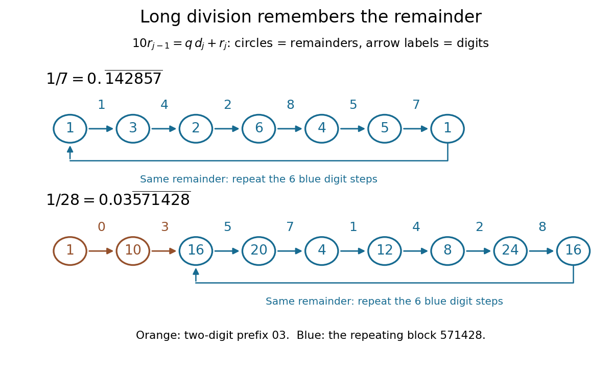
Long-division remainders explain the six-digit repeat of one seventh and the two-digit prefix of one twenty-eighth
. Details. More generally, initialize long division with . At each step, division with remainder givesso . Since are coprime integers, the modular inverse of shows that exactly when . To see why the digit block cannot repeat sooner than the remainders, a purely repeating decimal with a block of digits represents for an integer . A reduced fraction with that value forces . Hence the shortest digit repeat and the multiplicative order coincide.
Knowing the decimal period predicts how many digits must be computed and stored: one block determines the whole repeating decimal. It also constructs the block directly. With , the integeris the block, padded on the left with zeros to digits. For , and , so the block is and . Reduction matters: has decimal period one, whereas .
If the reduced denominator contains prime factors two or five, ten has no multiplicative order modulo that whole denominator. WriteThe decimal preperiod has exactly digits. If , the remaining repeating decimal has decimal period . For instance, gives : two prefix digits, then six repeating digits. If , the decimal representation is a terminating decimal with exactly fractional places. We use the representation ending in zeros, rather than its alternative ending in nines; for example terminates after three places.
A short derivation explains both cases. After digits, multiplying the reduced fraction by and discarding its integer part leaves a reduced fraction whose denominator is . This denominator first becomes coprime to ten at . It then equals , giving an immediate repeat when , or an integer when . The same long division argument works for positional notation in any base : for a reduced denominator coprime to , the shortest repeating block has length .
The product of numbers is the result of their iterated multiplication. The empty product is , the multiplicative identity. For positive factors, , turning a multiplicative conservation law into an additive derivative identity.
Electron affinity measures how strongly an isolated neutral species binds an additional electron. In the spectroscopic convention used here, it is the positive energy required to detach that electron from a bound anion. With the free electron at rest assigned zero energy,The quantum states of and must be specified, usually their ground states. Positive means that attachment lowers the energy; a signed attachment energy is then negative. This convention agrees with the IUPAC definition and with the atomic tables used for Mulliken electronegativity.[ref]
For chlorine, a published photodetachment threshold is , approximately per chemical atom. Here is the Planck constant, the speed of light, and the inverse-length unit expresses an energy through a spectroscopic wavenumber. The parentheses give the reported uncertainty in the last digits, not a range of possible sign conventions.[ref]
Isotope shift in the electron affinity of chlorine by U. Berzinsh and others. §2.3, printed pp. 6–7: reported threshold 29138.59(22) inverse centimetres
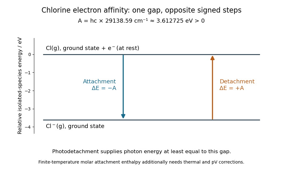
Electron affinity of chlorine: positive detachment energy and negative attachment energy connect the same isolated-species levels; a finite-temperature electron attachment enthalpy needs additional corrections
. Details. An electron affinity is neither an electronegativity nor a lattice energy. The first describes a specified isolated-species energy difference, electronegativity compares attraction for electron density in a chemical bond, and lattice energy refers to an entire ionic crystal and separated gaseous ions. A stable anion can therefore help explain ionic bonding without describing the full energy balance for making a salt.
To calculate , generate independent with density and average . Integrability gives convergence by the strong law of large numbers; finite variance gives an unbiased estimate with variance . Applying this to indicators estimates probabilities. Correlated Markov chain Monte Carlo samples can also approximate the integral, but their error is determined by the chain's dependence rather than the independent-sample variance formula.
A pseudorandom number generator is a deterministic state-update algorithm producing numbers intended to imitate an independent sequence from a prescribed probability distribution. For Monte Carlo integration, desirable features include good one-dimensional and multidimensional uniformity, a period far longer than the calculation, negligible detectable dependence, reproducible seeds, sufficient numerical precision and fast generation. Uniform marginal distributions alone do not provide independent draws.
The specific growth rate is biomass production per unit existing biomass per unit time. For biomass concentration with growth alone, and . A constant positive specific growth rate produces exponential growth, , with doubling time . In a chemostat, removal makes the net rate , rather than itself.
Occupying an antibonding molecular orbital opposes a chemical bond. For equivalent atomic orbitals of the hydrogen atom, the difference vanishes on the plane halfway between the protons: every point there is equally far from both centres, so the amplitudes cancel. This nodal plane removes the contribution of this molecular orbital to electron density on that plane; it does not make an entire finite region empty. The -derived antibonding molecular orbital lies above its bonding molecular orbital partner in energy. See Field, MIT 5.61, lecture 25, pp. 1–2.
In the minimal model, adds and cancels the bond order contribution of . Opposite signs on the two lobes describe probability amplitudes, while both lobes have nonnegative probability density after squaring. The star is an orbital label, not an extra electron or an electric charge.
Occupying a bonding molecular orbital favours a chemical bond. For the two equivalent atomic orbitals of the hydrogen atom, the sum has constructive interference between the protons. The resulting electron density in that region helps stabilize the combined system. Its lower energy in this model follows from the Quantum Hamiltonian, not from the plus sign alone; see Field, MIT 5.61, lecture 25, pp. 1–2.
For example, in molecular hydrogen supplies , hence bond order one when . The sum in the molecular orbital theory toy has midpoint probability density , whereas the difference has zero there. The normalization factors must be included in this comparison.
Pinned article: Introduction to the OurBigBook Project
Welcome to the OurBigBook Project! Our goal is to create the perfect publishing platform for STEM subjects, and get university-level students to write the best free STEM tutorials ever.
Everyone is welcome to create an account and play with the site: ourbigbook.com/go/register. We belive that students themselves can write amazing tutorials, but teachers are welcome too. You can write about anything you want, it doesn't have to be STEM or even educational. Silly test content is very welcome and you won't be penalized in any way. Just keep it legal!
Intro to OurBigBook
. Source. We have two killer features:
- topics: topics group articles by different users with the same title, e.g. here is the topic for the "Fundamental Theorem of Calculus" ourbigbook.com/go/topic/fundamental-theorem-of-calculusArticles of different users are sorted by upvote within each article page. This feature is a bit like:
- a Wikipedia where each user can have their own version of each article
- a Q&A website like Stack Overflow, where multiple people can give their views on a given topic, and the best ones are sorted by upvote. Except you don't need to wait for someone to ask first, and any topic goes, no matter how narrow or broad
This feature makes it possible for readers to find better explanations of any topic created by other writers. And it allows writers to create an explanation in a place that readers might actually find it.
Figure 1. Screenshot of the "Derivative" topic page. View it live at: ourbigbook.com/go/topic/derivativeVideo 2. OurBigBook Web topics demo. Source. - local editing: you can store all your personal knowledge base content locally in a plaintext markup format that can be edited locally and published either:This way you can be sure that even if OurBigBook.com were to go down one day (which we have no plans to do as it is quite cheap to host!), your content will still be perfectly readable as a static site.
- to OurBigBook.com to get awesome multi-user features like topics and likes
- as HTML files to a static website, which you can host yourself for free on many external providers like GitHub Pages, and remain in full control

Figure 2. You can publish local OurBigBook lightweight markup files to either OurBigBook.com or as a static website.
Figure 3. Visual Studio Code extension installation.
Figure 5. . You can also edit articles on the Web editor without installing anything locally. Video 3. Edit locally and publish demo. Source. This shows editing OurBigBook Markup and publishing it using the Visual Studio Code extension. 
- Infinitely deep tables of contents:




All our software is open source and hosted at: github.com/ourbigbook/ourbigbook
Further documentation can be found at: docs.ourbigbook.com
Feel free to reach our to us for any help or suggestions: docs.ourbigbook.com/#contact