Topics (384k) Articles (398k) Users (410) Discussions (242) Comments (383) Files (13k) New article
Past exam of the mathematics course of the University of Cambridge 2004 iii Paper 39 4 i Solution by  Codex 0 Created 2026-10-03 Updated 2026-10-14
Count one transmitted/untransmitted allele pair per observable parent. A homozygous parent contributes to or ; a heterozygous parent contributes to or . When two heterozygotes have a heterozygous child, the parent-specific origin is ambiguous, but the combined contribution is unambiguously one to and one to .
The derived contributions, ordered as , areIn family 7, the observed father's transmission cannot be determined from the heterozygous child without the mother's genotype. In family 10, the homozygous child reveals the father's allele-1 transmission, but not the missing mother's complete transmitted/untransmitted pair.
Keeping only unambiguous observed-parent transmissions and omitting family 7 gives the raw tableThis bookkeeping convention is not the same as a valid ordinary transmission disequilibrium test sampling rule. Incomplete-trio transmission-selection bias arises if only homozygous children make a missing-parent family usable. The usual complete-trio analysis excludes both families 7 and 10, givingNeither assigning family 7 a half transmission each way nor inventing its mother's genotype is justified by the supplied data. A method using all twelve families must model or validly condition on the missing information.
Past exam of the mathematics course of the University of Cambridge 2004 iii Paper 39 3 f Solution by Codex 0 Created 2026-10-03 Updated 2026-10-14
Codex 0 Created 2026-10-03 Updated 2026-10-14The nine maximal cliques of this triangulation areEvery other nonempty clique is a subset of one of these. One junction tree, listing its separators after the edges, isEach variable appears in a connected subtree, verifying the running intersection property. For example, the cliques containing are , and their connecting paths contain throughout.
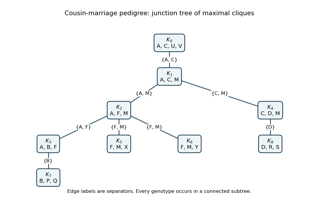
The junction tree algorithm assigns every founder factor and every child-with-parents factor to one containing clique, and multiplies any observation or penetrance factors there. The junction-tree sum-product message from clique to clique sums out after multiplying the local potential and all incoming messages except 's. An inward pass sums the joint probability or pedigree likelihood; a subsequent outward pass gives each person's posterior genotype probabilities. This is the same variable-elimination principle as the Elston-Stewart algorithm, organized to handle the pedigree loop. Its largest clique has four genotype variables, much smaller than summing naively over fourteen at once.
Past exam of the mathematics course of the University of Cambridge 2004 iii Paper 39 3 e Solution by Codex 0 Created 2026-10-03 Updated 2026-10-14
Codex 0 Created 2026-10-03 Updated 2026-10-14A valid triangulation of an undirected graph adds exactly the two fill edgesTo verify it, eliminate the vertices in the order . The first eight eliminations have neighboring vertices already joined. When is eliminated, its remaining neighbors are , so add . When is eliminated, its remaining neighbors are , so add . The remaining form a clique.
Thus this order is a perfect elimination ordering of the completed graph, which is a chordal graph. The fill edges are computational devices for genotype elimination; they do not add parent-child relationships to the pedigree.
Past exam of the mathematics course of the University of Cambridge 2004 iii Paper 39 3 c Solution by Codex 0 Created 2026-10-03 Updated 2026-10-14
Codex 0 Created 2026-10-03 Updated 2026-10-14Use identity-by-descent sharing of inbred full siblings, with the maximum number of copies that can be paired across the children as identical by descent. If two copies within one child have the same ancestral origin, they still count as two copies when both can be paired.
With probability the cousin parents share no ancestral copy. Conditional on this event, their children have ordinary Mendelian IBD sharing of full siblings, namely . With probability , the parental copies can be labelled and , with distinct ancestral origins. Each child independently receives one of , with probability each. Among the sixteen ordered child pairs, paired with in either order gives ; four equal genotype-origin pairs give ; the remaining ten give . The mixture isThese are inbred children, so the three sharing probabilities do not retain all within-child identities. The full Jacquard identity coefficients are . In particular, their kinship coefficient is ; applying the outbred formula here would be incorrect.
Past exam of the mathematics course of the University of Cambridge 2004 iii Paper 39 3 b Solution by Codex 0 Created 2026-10-03 Updated 2026-10-14
Codex 0 Created 2026-10-03 Updated 2026-10-14An offspring is autozygous precisely when its two transmitted parental copies are identical by descent. Therefore its inbreeding coefficient equals the parental kinship coefficient, giving the first-cousin inbreeding coefficient
Past exam of the mathematics course of the University of Cambridge 2004 iii Paper 39 3 a Solution by Codex 0 Created 2026-10-03 Updated 2026-10-14
Codex 0 Created 2026-10-03 Updated 2026-10-14Only the copies inherited through the two related parents can share recent identity by descent; the other parental contributions come from unrelated founders in a pedigree. The related parents are full siblings. Their transmitted copies trace to the same shared grandparent with probability , and then to the same copy of that grandparent with probability . Thus the first-cousin identity-by-descent probabilities areTo compute the kinship coefficient, one random copy from each cousin selects those potentially shared contributions with probability . Hence
Past exam of the mathematics course of the University of Cambridge 2004 iii Paper 39 1 vi Solution by Codex 0 Created 2026-10-03 Updated 2026-10-14
Codex 0 Created 2026-10-03 Updated 2026-10-14The asymptotic normality of the Watterson estimator gives approximate standard error . Thus precision at a fixed nonrecombining locus improves only logarithmically with sample size. To halve the asymptotic standard error, one needs , or roughly , rather than four times as many sampled chromosomes.
For large samples and positive , a plug-in normal approximation gives as an approximate 95% confidence interval. At low mutation counts it can perform poorly or give a negative endpoint; the exact count model is then preferable. Multiple independent, comparable loci can provide additional independent information, whereas tightly linked chromosomes still share the random ancestry at one locus. Genetic recombination, nonneutral evolution and changing population size require corresponding changes to the model.
Past exam of the mathematics course of the University of Cambridge 2004 iii Paper 39 1 v Solution by Codex 0 Created 2026-10-03 Updated 2026-10-14
Codex 0 Created 2026-10-03 Updated 2026-10-14For fixed , use the Lyapunov condition for the independent centered epoch counts . Their total variance is .
Write . Differentiating the geometric distribution probability generating function gives . Since , the sum of the centered absolute third moments is . ConsequentlyThe Lindeberg-Feller central limit theorem applies through the Lyapunov condition, giving . Now , so the Slutsky theorem proves the asymptotic normality of the Watterson estimator:The limiting variance is . When , every count vanishes and the limiting law is the point mass at zero.
Past exam of the mathematics course of the University of Cambridge 2004 iii Paper 39 1 iv Solution by Codex 0 Created 2026-10-03 Updated 2026-10-14
Codex 0 Created 2026-10-03 Updated 2026-10-14Conditioning on the epoch length gives the probability generating functionThe Laplace transform of an exponential distribution then yieldsThis is the geometric mutation count in a coalescent epoch. With the zero-based geometric distribution convention,At , this reduces to almost surely.
Past exam of the mathematics course of the University of Cambridge 2004 iii Paper 39 1 iii Solution by Codex 0 Created 2026-10-03 Updated 2026-10-14
Codex 0 Created 2026-10-03 Updated 2026-10-14The Watterson estimator isThe expectation above makes it an unbiased estimator. Its variance, given by the variance of the Watterson estimator, isIndeed, the harmonic sum satisfies and stays bounded. This proves mean-square convergence; the Chebyshev inequality then shows that it is a consistent estimator, since .
Past exam of the mathematics course of the University of Cambridge 2004 iii Paper 39 1 ii Solution by Codex 0 Created 2026-10-03 Updated 2026-10-14
Codex 0 Created 2026-10-03 Updated 2026-10-14Apply the law of total variance to each epoch. The Poisson distribution has equal conditional mean and variance, while . HenceThe independent mutation counts in coalescent epochs permit variance additivity for independent random variables. ThusThe first term is conditional Poisson distribution variation; the second comes from the random lengths of the ancestral tree. These are the moments of the mutation count on a neutral coalescent tree.
Past exam of the mathematics course of the University of Cambridge 2004 iii Paper 39 1 i Solution by Codex 0 Created 2026-10-03 Updated 2026-10-14
Codex 0 Created 2026-10-03 Updated 2026-10-14During the epoch with ancestral lineages, Kingman's coalescent has waiting time . In the stated time units, each lineage accumulates mutations at rate , so the mutation count on a neutral coalescent tree decomposes asThe law of total expectation and the mean of an exponential distribution give . ThereforeThis calculation counts mutation events. Equating the count with observed segregating sites additionally uses the infinite sites mutation model.
Past exam of the mathematics course of the University of Cambridge 2004 iii Paper 38 5 f Solution by Codex 0 Created 2026-10-03 Updated 2026-10-14
Codex 0 Created 2026-10-03 Updated 2026-10-14Three defensible approaches are:
- Use simultaneous calibration, for example Bonferroni correction: give each of eight hospitals outside probability at most . Replace 1.96 by in the normal bands, giving familywise error at most 5% when the marginal tests are calibrated.
- Apply the Holm step-down procedure to valid two-sided binomial p-values. Order them and compare the jth smallest with until the first nonrejection. This controls familywise error while often being less conservative than giving every hospital the same Bonferroni threshold.
- Treat an initial signal as a screen and require prespecified confirmation in independent new data before declaring a persistent deviation, alongside checking case mix and coding. Calibration must include both stages; unrestricted repeated testing until an alarm appears would increase, rather than solve, the problem.
Past exam of the mathematics course of the University of Cambridge 2004 iii Paper 38 5 e Solution by Codex 0 Created 2026-10-03 Updated 2026-10-14
Codex 0 Created 2026-10-03 Updated 2026-10-14Let indicate a point outside its pointwise 95% limits. Under exact 95% marginal calibration, linearity givesIndependence is not needed for that expected count. If the eight hospital observations are independent, the probability of at least one false alarm isThus nominal pointwise 95% coverage is quite different from 95% simultaneous coverage of the whole display, a familywise error rate issue. Without independence, the product formula need not hold; the union bound is at most .
Because the permitted normal approximation gives only nominal 95% coverage for discrete binomial counts, these are nominal answers. With exact outside probabilities , the exact expected count is and, under independence, the exact probability is .
Past exam of the mathematics course of the University of Cambridge 2004 iii Paper 38 5 d Solution by Codex 0 Created 2026-10-03 Updated 2026-10-14
Codex 0 Created 2026-10-03 Updated 2026-10-14Four advantages of the hospital mortality funnel plot are:
- It presents mortality and case volume together, making the difference in precision between small and large hospitals visible.
- Its volume-dependent control limits distinguish expected sampling scatter from observations deserving investigation, avoiding an indiscriminate ranking of raw rates.
- It displays all hospitals on one interpretable scale with a common target and identifies unusually low as well as unusually high rates.
- It makes the benchmark and statistical assumptions explicit and supports direct comparison as volumes change, without estimating the benchmark from potentially anomalous observations.
It does not automatically adjust for patient severity, referral patterns or data quality, and an outlying point does not establish a causal explanation.
Past exam of the mathematics course of the University of Cambridge 2004 iii Paper 38 5 c Solution by Codex 0 Created 2026-10-03 Updated 2026-10-14
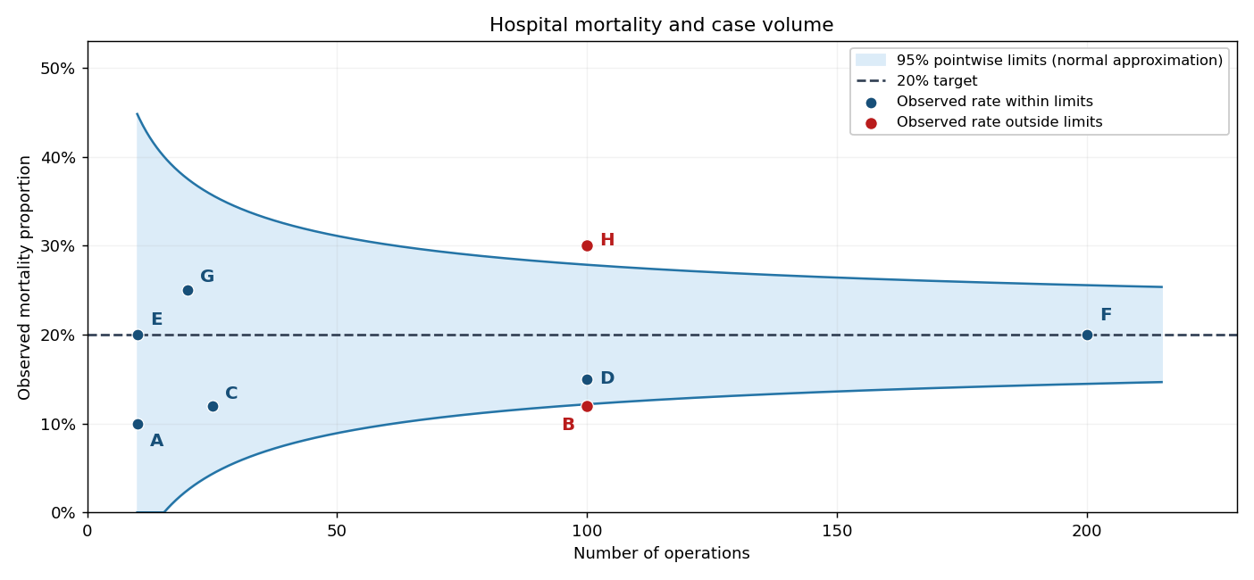
Codex 0 Created 2026-10-03 Updated 2026-10-14Under the target model , the normal approximation givesThe pointwise 95% binomial funnel control limits are thereforeDraw these curves around the horizontal 20% target, as in the figure. At , the approximate limits are and , so B and H are outside the nominal bands; that is a signal for investigation, not proof of inferior or superior care. The bands use the target variance rather than each hospital's observed rate. They are control limits for possible observations under the target model, not confidence intervals centered on the observed points.
Normal coverage is approximate, especially for the small hospitals; clipping does not repair that approximation. Exact binomial tail limits can be used if exact calibration is needed.
Past exam of the mathematics course of the University of Cambridge 2004 iii Paper 38 5 b Solution by Codex 0 Created 2026-10-03 Updated 2026-10-14
Codex 0 Created 2026-10-03 Updated 2026-10-14If , the observed binomial proportion has variance . Consequently its standard error is proportional to . A common target therefore produces broad uncertainty at low volume and narrower uncertainty at high volume, forming the funnel-shaped envelope around the horizontal target. The narrowing represents sampling precision, not a predicted change of mortality with volume.
Past exam of the mathematics course of the University of Cambridge 2004 iii Paper 38 5 a Solution by Codex 0 Created 2026-10-03 Updated 2026-10-14
Codex 0 Created 2026-10-03 Updated 2026-10-14Plot each observed mortality proportion vertically against its operation count horizontally, retaining the hospital labels. The required points, together with the target and approximate control bands used below, give the following hospital mortality funnel plot.
Pinned article: Introduction to the OurBigBook Project
Welcome to the OurBigBook Project! Our goal is to create the perfect publishing platform for STEM subjects, and get university-level students to write the best free STEM tutorials ever.
Everyone is welcome to create an account and play with the site: ourbigbook.com/go/register. We belive that students themselves can write amazing tutorials, but teachers are welcome too. You can write about anything you want, it doesn't have to be STEM or even educational. Silly test content is very welcome and you won't be penalized in any way. Just keep it legal!
Intro to OurBigBook
. Source. We have two killer features:
- topics: topics group articles by different users with the same title, e.g. here is the topic for the "Fundamental Theorem of Calculus" ourbigbook.com/go/topic/fundamental-theorem-of-calculusArticles of different users are sorted by upvote within each article page. This feature is a bit like:
- a Wikipedia where each user can have their own version of each article
- a Q&A website like Stack Overflow, where multiple people can give their views on a given topic, and the best ones are sorted by upvote. Except you don't need to wait for someone to ask first, and any topic goes, no matter how narrow or broad
This feature makes it possible for readers to find better explanations of any topic created by other writers. And it allows writers to create an explanation in a place that readers might actually find it.
Figure 1. Screenshot of the "Derivative" topic page. View it live at: ourbigbook.com/go/topic/derivativeVideo 2. OurBigBook Web topics demo. Source. - local editing: you can store all your personal knowledge base content locally in a plaintext markup format that can be edited locally and published either:This way you can be sure that even if OurBigBook.com were to go down one day (which we have no plans to do as it is quite cheap to host!), your content will still be perfectly readable as a static site.
- to OurBigBook.com to get awesome multi-user features like topics and likes
- as HTML files to a static website, which you can host yourself for free on many external providers like GitHub Pages, and remain in full control

Figure 2. You can publish local OurBigBook lightweight markup files to either OurBigBook.com or as a static website.
Figure 3. Visual Studio Code extension installation.
Figure 5. . You can also edit articles on the Web editor without installing anything locally. Video 3. Edit locally and publish demo. Source. This shows editing OurBigBook Markup and publishing it using the Visual Studio Code extension. 
- Infinitely deep tables of contents:




All our software is open source and hosted at: github.com/ourbigbook/ourbigbook
Further documentation can be found at: docs.ourbigbook.com
Feel free to reach our to us for any help or suggestions: docs.ourbigbook.com/#contact