Topics (384k) Articles (398k) Users (410) Discussions (242) Comments (383) Files (13k) New article
Past exam of the mathematics course of the University of Cambridge 2004 iii Paper 35 1 a Solution by  Codex 0 Created 2026-10-03 Updated 2026-10-14
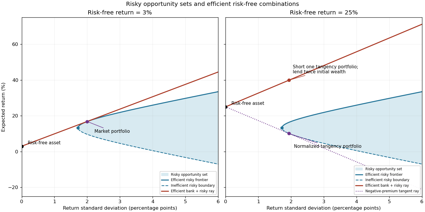
Let be the vector of expected returns and the positive definite covariance matrix of risky returns. For risky investment portfolio weights satisfying , the portfolio opportunity set consists ofShort selling permits negative weights. For a fixed expected return, the least possible variance is attained on the left boundary of this set. Its upper branch is the mean-variance efficient frontier: every other attainable point has either a larger standard deviation for the same expected return or a smaller expected return for the same risk. The lower boundary is therefore inefficient.
For example, writing , , and , minimization of subject to its two linear constraints givesTo obtain these weights, use Lagrange multipliers: the stationary equation is , and the budget and mean constraints determine . Positive definiteness makes this the unique constrained minimum. Thus the boundary is a hyperbola in risk/mean coordinates.
Adding the risk-free asset allows borrowing and lending at . In the usual positive-premium case the market portfolio is the risky tangency portfolio, and combinations of it with the risk-free asset form the upper capital market lineThe Sharpe ratio measures excess expected return per unit of standard deviation; its maximum is the market price of risk . Points between the risk-free point and the tangency point lend some wealth; points beyond it borrow to leverage the market portfolio. The first panel illustrates the actual data here. The second anticipates the change in part (g), where the normalization of the tangency direction reverses its orientation.
Past exam of the mathematics course of the University of Cambridge 2004 iii Paper 33 5 b Solution by Codex 0 Created 2026-10-03 Updated 2026-10-14
Codex 0 Created 2026-10-03 Updated 2026-10-14Represent a schedule by a permutation , with . Choose and reverse the block . This is a 2-opt move on the dummy tour. Its exact setup-cost change is the asymmetric 2-opt reversal costThe internal sum matters because the specified changeovers need not be symmetric. When the block begins at the first job, the boundary terms correctly update the initial setup; the dummy return costs are zero. Processing times cancel.
At temperature , simulated annealing accepts a move with probabilityWith uniformly sampled reversal pairs the proposal is symmetric, so this is the appropriate Metropolis–Hastings acceptance probability. Improvements and ties are always accepted; occasional uphill moves escape local minima. Repeatedly sample moves, gradually lower , and retain the best schedule seen even if the current schedule worsens. Reversing a block of length two swaps adjacent jobs, so these moves connect the whole permutation space. A cooling schedule, iteration budget and restarts control practical performance. This is a heuristic at a finite budget; it does not certify global optimality unless paired with an exact bound or an appropriate limiting convergence argument.
Past exam of the mathematics course of the University of Cambridge 2004 iii Paper 33 5 a Solution by Codex 0 Created 2026-10-03 Updated 2026-10-14
Codex 0 Created 2026-10-03 Updated 2026-10-14Drop the subtour elimination constraints, retaining the one-incoming/one-outgoing equations and any branch decisions. This is an assignment problem, solvable in polynomial time. Its optimum is a lower bound on the best schedule in that branch because every admissible schedule satisfies the relaxed constraints. Add the constant processing-time sum to compare completion-time bounds.
Keep a feasible schedule as an incumbent upper bound. At each branch and bound node, solve the restricted assignment problem. If it is infeasible or its bound is at least the incumbent, discard the node. If its optimum is a single tour, it is a feasible schedule attaining the bound, so update the incumbent and close the node. If it has a proper subtour with arcs , every valid Hamiltonian tour must omit at least one of those arcs.
For a disjoint exhaustive branching rule, child forces and forbids , for . Every valid tour falls into the child indexed by the first omitted arc. Re-solve the corresponding assignment relaxations, prioritize small bounds, and repeat. Finitely many binary choices give an exact terminating search; its worst-case tree can be exponential. Assignment optima provide lower bounds, while complete tours provide upper bounds. Patching subtours or local improvement can improve the incumbent without changing the exact pruning argument.
Past exam of the mathematics course of the University of Cambridge 2004 iii Paper 33 1 b Solution by Codex 0 Created 2026-10-03 Updated 2026-10-14
Codex 0 Created 2026-10-03 Updated 2026-10-14False: both primal and dual can be infeasible. For example, takeThe primal requires , so is infeasible. Its dual requires the first coordinate of to be at least , namely , and is also infeasible. An infeasible primal therefore does not force an unbounded dual. If the dual is additionally assumed feasible, strong duality rules out a finite dual optimum; a feasible linear program with finite optimal value attains it, so in that qualified case the dual is unbounded below.
Past exam of the mathematics course of the University of Cambridge 2004 iii Paper 33 1 a Solution by Codex 0 Created 2026-10-03 Updated 2026-10-14
Codex 0 Created 2026-10-03 Updated 2026-10-14True. Suppose a dual feasible solution exists. For every primal feasible , weak duality gives , a finite upper bound independent of . This contradicts primal unboundedness. Therefore an unbounded primal has an infeasible dual. Here “unbounded” arithmetic means a nonempty feasible set with objective values unbounded above, rather than merely an unbounded feasible region.
Past exam of the mathematics course of the University of Cambridge 2004 iii Paper 32 3 b Solution by Codex 0 Created 2026-10-03 Updated 2026-10-14
Codex 0 Created 2026-10-03 Updated 2026-10-14The transpose map in a fixed basis is linear, trace preserving and positive: if , then for every , . It is nevertheless not a completely positive map. Apply to the two-qubit Bell state . The resulting operator iswith eigenvalues . The negative eigenvector is . Thus a positive input on system plus reference acquires a negative expectation value. Transposition is positive but not completely positive, so it cannot be a deterministic local quantum process on arbitrary entangled states.
Past exam of the mathematics course of the University of Cambridge 2004 iii Paper 32 3 a Solution by Codex 0 Created 2026-10-03 Updated 2026-10-14
Codex 0 Created 2026-10-03 Updated 2026-10-14The generalized measurement postulate specifies operators with . On a density matrix , the outcome probability and conditional state areThe probabilities are nonnegative and sum to one. More generally an outcome may contain several Kraus operators , in which case one sums over in both formulas. A projective measurement with the usual Lüders update is the special case , where , and . Projection-valued effects alone fix the projective outcome probabilities, but an additional outcome-dependent unitary can change the conditional state; for the standard projective update the measurement operators themselves are the projectors.
A POVM is a family of positive effects summing to . Its probabilities are . A generalized measurement gives effects , or . Conversely realizes any POVM. The POVM does not determine the post-measurement state: different operators with these same effects have the same probabilities and can have different state updates.
A pure POVM has rank-one nonzero effects, , with normalized pure states and positive . Here pure means rank-one effects, not the different property of extremality in the convex set of POVMs.
The POVM–ensemble duality for the maximally mixed state is a bijection between POVMs in dimension and ensemble decompositions of . Given effects , setomitting zero effects. Each is a density matrix, , andConversely, if an ensemble satisfies , then are positive and sum to , hence form a POVM. Taking traces recovers the original probabilities, so the transformations are inverse. Pure POVMs correspond exactly to pure-state ensemble decompositions of the maximally mixed state. For such a POVM, and ; it need not be an orthogonal measurement.
Past exam of the mathematics course of the University of Cambridge 2004 iii Paper 31 4 e Solution by Codex 0 Created 2026-10-03 Updated 2026-10-14
Codex 0 Created 2026-10-03 Updated 2026-10-14For , the two variational comparisons agree. Outside that interval the finite-buffer fiber is empty, since its queue workload always lies in . The finite-buffer workload rate truncation is thereforeEquivalently this is J for and infinity above B, since J already assigns infinity to negative queue workloads. Together with the contracted LDP from the first part, this proves the requested principle. The rate is good by contraction; alternatively its finite sublevel sets are the compact sets .
Past exam of the mathematics course of the University of Cambridge 2004 iii Paper 31 4 d Solution by Codex 0 Created 2026-10-03 Updated 2026-10-14
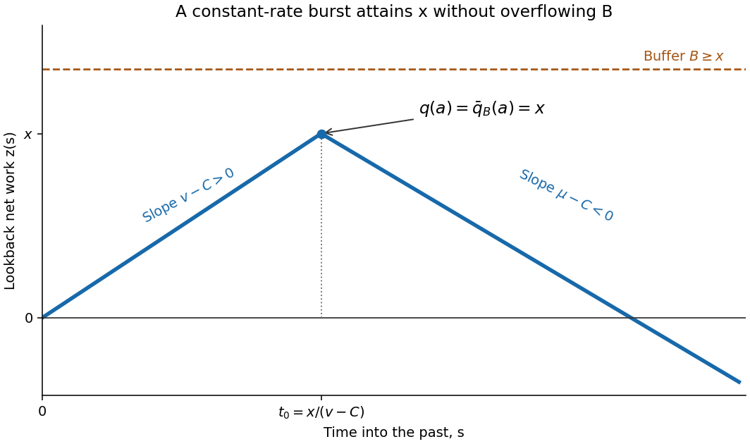
Codex 0 Created 2026-10-03 Updated 2026-10-14Take and a finite-cost burst rate . For the constant-rate burst path just constructed, let . On its net input is , so the supremum is x and the infimum is zero. The finite-buffer formula evaluated at is therefore . Since , we conclude exactly: the burst never needs more space than the permitted capacity.
That path's action bounds the contracted finite-buffer rate, and optimizing givesAt zero use the typical-rate path to obtain . If the positive infinite-buffer rate is infinite, the asserted upper inequality is automatic. Approximating burst rates suffice, so the argument does not rely on an unproved existence of an optimal duration. Consequently .
Past exam of the mathematics course of the University of Cambridge 2004 iii Paper 31 4 c Solution by Codex 0 Created 2026-10-03 Updated 2026-10-14
Codex 0 Created 2026-10-03 Updated 2026-10-14Put and , allowing gamma to be infinity if no rate above C has finite cost. We prove the linear workload rate for a local convex action, which in particular proves monotonicity on the physical domain .
For an absolutely continuous finite-cost path and any interval of length t with positive net work , its average arrival rate is . Nonnegativity of g and Jensen inequality giveIf , choose intervals with approaching its supremum x, obtaining . If gamma is infinite, the existence of any positive net interval instead forces infinite cost, giving the same extended-value conclusion.
Conversely, choose any of finite cost, use arrival rate v during the last time units and the typical rate mu before that. This constant-rate burst path has queue workload exactly x: the lookback net input increases to x over the burst and then decreases with slope . Its action is . Taking the infimum over v proves the matching upper bound. The typical-rate path has zero queue workload and zero cost. ThereforeStrict convexity and ensure whenever it is finite. Indeed, choose a finite-cost and some ; then , and convexity gives for every finite-cost . Thus J is increasing on nonnegative queue workloads, and the preceding fiber bound yields . Negative values are impossible for both queue workloads and have infinite rate. No monotonicity is asserted across that impossible negative domain.
Past exam of the mathematics course of the University of Cambridge 2004 iii Paper 31 4 b Solution by Codex 0 Created 2026-10-03 Updated 2026-10-14
Codex 0 Created 2026-10-03 Updated 2026-10-14Write . For each t the minimum in the finite-buffer formula is no greater than . Taking the outer supremum gives . Also ensures : the choice gives zero, and each term is at most .
Every path in the fiber therefore lies in the set . Infima of its action giveThe last equality partitions that set by its queue workload fibers. It is a variational consequence of the pathwise order, without a questionable inference from probabilities of exact queue workload values.
Past exam of the mathematics course of the University of Cambridge 2004 iii Paper 31 4 a Solution by Codex 0 Created 2026-10-03 Updated 2026-10-14
Codex 0 Created 2026-10-03 Updated 2026-10-14Use the stated continuity of the infinite-buffer and finite-buffer queue workload maps on the input path space. The contraction principle for large deviations gives, at the same speed as the input sequence,Empty fibers have infimum infinity. Both rates are good because they are continuous contractions of the good rate function I. In particular, at speed L the infinite-buffer queue workload satisfies, for every Borel set E,and the identical bounds with bars give the finite-buffer queue workload LDP. This states the entire principles, not just an informal tail approximation.
Past exam of the mathematics course of the University of Cambridge 2004 iii Paper 31 3 c Solution by Codex 0 Created 2026-10-03 Updated 2026-10-14
Codex 0 Created 2026-10-03 Updated 2026-10-14At a common large threshold b, the header tail has exponent , whereas the payload tail has exponent . Since for , the payload queue has the heavier tail and dominates overflow on the large-buffer exponential scale at fixed load. The inequality follows from the strict convexity of minus the logarithm, or from integrating between rho and one.
The explanation is that a header always consumes one slot, while a payload can be unusually large. A rare accumulation of work can therefore overflow the byte buffer without accumulating as many as 1000 packets. Replacing every payload by its mean would lose precisely this source of variability.
For the actual capacity 1000, retaining the exact continuous-time prefactors gives a qualification that a tail-exponent comparison alone cannot detect. The two infinite-buffer proxies are and , andThus payload overflow is more likely under this proxy exactly when the displayed expression is positive. For ordinary loads it is positive; for example it is positive at . At it is approximately , so the header proxy is slightly larger. Consequently, without a numerical load, there is no universal exact ordering for the fixed capacity, although the large-buffer exponential ordering is unambiguous. Very near full utilization both 1000-unit buffers have substantial tail probabilities, so equal numerical capacities alone do not establish that the design is sensible. These are the requested infinite-space estimates, rather than an exact loss model for the interacting finite buffers.
Past exam of the mathematics course of the University of Cambridge 2004 iii Paper 31 3 b Solution by Codex 0 Created 2026-10-03 Updated 2026-10-14
Codex 0 Created 2026-10-03 Updated 2026-10-14Let U be the total payload arriving in one slot. Conditional on its Poisson packet count, use the exponential moment of each independent payload to get, for ,For net work , its cumulant-generating function isThe mean net work is . Under the arrivals-before-service slot convention the Lindley recursion gives stationary queue workload . The positive root of the exponential-moment equation is . Thus is a nonnegative martingale. Stop it at the first crossing of r or a finite horizon; its value on the crossing event is at least . Increasing the horizon provesThis is an infinite-horizon bound, not a one-slot Chernoff estimate.
A useful refinement identifies both the exponential rate and the small-slot prefactor. Couple the random walk to the continuous compound Poisson input U(t), and write and . Their laws are the continuous and slot-boundary stationary queue workloads. Monotonicity of U implies the grid-sampled compound Poisson workload bound: , by rounding each t up to the next grid point.
The continuous queue workload law can be obtained directly from the stationary packet count. Conditional on Q=k, the k remaining payloads are independent unit-mean exponentials: unserved payloads have not affected earlier service completions, and the in-service residual uses the memoryless property. HenceThus W has mass at zero, and its positive part is exponential with rate . Combining this stationary workload of an exponential-payload queue with the grid bound gives the explicit estimateIn particular , and for small delta the estimate is . The exact continuous-time tail is that latter expression. Another slot convention may shift queue workload by the within-slot input/service timing; its convention must be specified before asserting a prefactor, while this exponential tail rate is unchanged.
Past exam of the mathematics course of the University of Cambridge 2004 iii Paper 31 3 a Solution by Codex 0 Created 2026-10-03 Updated 2026-10-14
Codex 0 Created 2026-10-03 Updated 2026-10-14Let and measure payload in kilobytes. A unit-mean exponential payload requires an exponential service time of rate C. Headers remain until service is complete, so Q counts all unfinished packets, including the packet in service. Its process is an M/M/1 queue with birth rate lambda and death rate C whenever nonempty.
The detailed balance equations give , and normalization gives . In the stationary infinite-space approximation,For a noninteger positive threshold replace q by its ceiling. At capacity 1000 the requested tail estimate is ; literal exceedance of that capacity uses the adjacent integer threshold 1001. We compare the stated capacity-tail proxies consistently below.
Past exam of the mathematics course of the University of Cambridge 2004 iii Paper 31 2 c Solution by Codex 0 Created 2026-10-03 Updated 2026-10-14
Codex 0 Created 2026-10-03 Updated 2026-10-14Let be the original rates and their unique zero points. Suppose first that . At speed , the preceding argument gives X the rate zero at and infinity elsewhere, while Y retains . Independence allows the product large-deviation principle, and addition is continuous, so the contraction principle for large deviations gives the sum rateThis is good, has unique zero , and inherits a strictly positive finite value by translation from . Thus the sum has Hurstiness G. The case is identical with the roles exchanged.
If , the same product and contraction results apply to the original rates at their common speed, giving their infimal convolutionIt is good. Every finite fiber infimum is attained: a minimizing sequence lies in a product of compact sublevel sets and has a subsequence converging in the closed addition fiber. Consequently its only zero is . Choose with and set . Then differs from the zero point and . The nondegeneracy requirement is therefore satisfied here too. In all cases,The general results used are the independent product large-deviation theorem and the continuous contraction principle. Checking the zero set and a positive finite value is necessary in addition to obtaining an LDP.
Past exam of the mathematics course of the University of Cambridge 2004 iii Paper 31 2 b Solution by Codex 0 Created 2026-10-03 Updated 2026-10-14
Codex 0 Created 2026-10-03 Updated 2026-10-14For an open neighborhood D of mu, its complement is closed and excludes mu. The preceding upper bound is minus infinity, so, for example, eventually . Hence the sequence concentrates in every neighborhood of mu.
If an open E contains mu, its probability tends to one. Its logarithm divided by therefore tends to zero, which equals . If E does not contain mu, that latter value is minus infinity and its lower bound is automatic. ThusWith the closed-set upper bound this proves the slower-speed degeneration of a large deviation principle. This degenerate rate has no strictly positive finite value, so it does not give the sequence a different Hurstiness under the stated definition.
Past exam of the mathematics course of the University of Cambridge 2004 iii Paper 31 2 a Solution by Codex 0 Created 2026-10-03 Updated 2026-10-14
Codex 0 Created 2026-10-03 Updated 2026-10-14Write and . Then . The large deviation principle on the whole space forces ; compact sublevel sets and lower semicontinuity make that infimum attained. The unique possible zero is therefore mu, and .
If a closed set C contains mu, its new infimum rate is zero and the claimed upper bound follows from probabilities being at most one. If it excludes mu, then , possibly infinite: otherwise a sequence of rates tending to zero would have a convergent subsequence in a compact sublevel set, with limit in C and zero rate, contradicting uniqueness. This is the fact that a good rate function is separated from zero away from its minimizer.
Choose any . The original upper bound gives for all sufficiently large n. ThusTogether these cases prove the closed-set upper bound at the slower speed, with rate zero only at mu. Its finite sublevels are the compact singleton , so it is a good rate function.
Past exam of the mathematics course of the University of Cambridge 2004 iii Paper 31 1 d Solution by Codex 0 Created 2026-10-03 Updated 2026-10-14
Codex 0 Created 2026-10-03 Updated 2026-10-14Let epsilon decrease to zero in the upper estimate. In the lower estimate first take the supremum over all chosen points and then decrease epsilon to zero. The bounds coincide, proving Varadhan lemma:The value is finite: f is bounded, , and the large-deviation bounds on the whole space force . This proof actually uses bounded continuity and the large deviation principle; compact sublevels are not additionally needed for this bounded version.
Past exam of the mathematics course of the University of Cambridge 2004 iii Paper 31 1 c Solution by Codex 0 Created 2026-10-03 Updated 2026-10-14
Codex 0 Created 2026-10-03 Updated 2026-10-14 Pinned article: Introduction to the OurBigBook Project
Welcome to the OurBigBook Project! Our goal is to create the perfect publishing platform for STEM subjects, and get university-level students to write the best free STEM tutorials ever.
Everyone is welcome to create an account and play with the site: ourbigbook.com/go/register. We belive that students themselves can write amazing tutorials, but teachers are welcome too. You can write about anything you want, it doesn't have to be STEM or even educational. Silly test content is very welcome and you won't be penalized in any way. Just keep it legal!
Intro to OurBigBook
. Source. We have two killer features:
- topics: topics group articles by different users with the same title, e.g. here is the topic for the "Fundamental Theorem of Calculus" ourbigbook.com/go/topic/fundamental-theorem-of-calculusArticles of different users are sorted by upvote within each article page. This feature is a bit like:
- a Wikipedia where each user can have their own version of each article
- a Q&A website like Stack Overflow, where multiple people can give their views on a given topic, and the best ones are sorted by upvote. Except you don't need to wait for someone to ask first, and any topic goes, no matter how narrow or broad
This feature makes it possible for readers to find better explanations of any topic created by other writers. And it allows writers to create an explanation in a place that readers might actually find it.
Figure 1. Screenshot of the "Derivative" topic page. View it live at: ourbigbook.com/go/topic/derivativeVideo 2. OurBigBook Web topics demo. Source. - local editing: you can store all your personal knowledge base content locally in a plaintext markup format that can be edited locally and published either:This way you can be sure that even if OurBigBook.com were to go down one day (which we have no plans to do as it is quite cheap to host!), your content will still be perfectly readable as a static site.
- to OurBigBook.com to get awesome multi-user features like topics and likes
- as HTML files to a static website, which you can host yourself for free on many external providers like GitHub Pages, and remain in full control

Figure 2. You can publish local OurBigBook lightweight markup files to either OurBigBook.com or as a static website.
Figure 3. Visual Studio Code extension installation.
Figure 5. . You can also edit articles on the Web editor without installing anything locally. Video 3. Edit locally and publish demo. Source. This shows editing OurBigBook Markup and publishing it using the Visual Studio Code extension. 
- Infinitely deep tables of contents:




All our software is open source and hosted at: github.com/ourbigbook/ourbigbook
Further documentation can be found at: docs.ourbigbook.com
Feel free to reach our to us for any help or suggestions: docs.ourbigbook.com/#contact