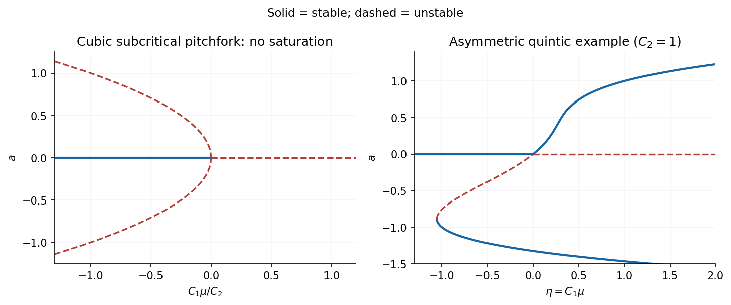
The quintic term points inward for sufficiently large ∣a∣, so all forward solutions are bounded and approach equilibria in this scalar problem. The quadratic term breaks a↦−asymmetry. Besides a=0, the equilibrium diagram is
η=g(a)=a−Ca2+a4,a nonzero equilibrium is stable iff ag′(a)>0.
This stability criterion follows from f′(a)=−ag′(a) on the equilibriumcurve, where g′=1−2Ca+4a3. Near zero the new branch is a=η+O(η2), crossing the trivial branch transcritically. It is unstable for small negative η and stable for small positive η; the trivial branch has the opposite stability.
The negative-amplitude part of g has exactly one minimum. Above its negative fold value but below zero, a stable finite-amplitude negative state coexists with the stable origin, separated by an unstable negative equilibrium. This gives hysteresis and finite-amplitude triggering of convection. For positive η the origin is unstable and stable nonzero states provide saturation. Additional positive-amplitude folds depend on C: g′ has two positive roots for C>3/2, adouble root at C=3/2 and none for C<3/2, so further multistability can occur. The right-hand figure illustrates C=1, without those extra positive folds; it does not assume that every possible C2 gives that same detailed diagram. These are the qualitative changes in quintic saturation of a symmetry-broken pitchfork.
Fix μ=r−1−q and 0<q<ζ/σ. The noncritical eigenvalues at μ=0 are −ζ and σq−ζ<0. Include the constant parameteras an additional centre variable. Symmetry permits expansions
where the omitted terms in the reduced equation have order μ2a,μa3,a5. At μ=0, a′ begins at cubic order, so c′=caa′ begins at fourth order. The cequation therefore gives c2=3/ζ2.
Both coefficients are positive. Thus the bifurcation is a subcritical pitchfork: the no-convection state is stable for μ<0 and unstable for μ>0. The small nonzero branches lie on the stable-origin side,
A zero eigenvalue occurs at r=1+q. If q<ζ/σ, the other two eigenvalues are negative, and the stationary bifurcation is the pitchfork analyzed in part (c). For q>ζ/σ the transverse eigenvalue is positive instead.
An imaginary pair occurs at r=1+ζ/σ, provided q>ζ/σ, because
The trace crosses zero with derivativeσ>0. The cubic coupling is nondegenerate here: at criticality, putting K=σζq reduces the oscillatory variables to
For a=Rcos(ωHτ), the forced secondharmonic of c has sinecoefficient 9R2ζωH/[2K(ζ2+4ωH2)]. Averaging the derivative of (a′2+ωH2a2)/2 consequently gives −9ζωH2R4/[8(ζ2+4ωH2)]<0. Thus the Hopf bifurcation is nondegenerate and supercritical.
Here the planar block is nonzero but has trace and determinant zero, while the third eigenvalue remains negative. It is a reflection-symmetric double-zero, codimension-two point; the ordinary simple-eigenvalue reduction of part (c) is not valid there.
Write α=π/3 and L=α2+π2=4π2/3. The primary streamfunction mode describes a single roll spanning the box, while the first magnetic mode describes the distortion of the vertical field by that roll. The second magnetic mode is independent of height and has twice the horizontal wavenumber, as generated by interaction of the first two modes. Take
For example the coefficient of a in b′ is (π/L)(42)/(32/π)=1, and that of ab in c′ is 3. The linear momentumcoefficients become r=Rα2/L3=9R/(64π4) and q=Qπ2/L2=9Q/(16π2). Therefore
Use a small incoming neighborhood of the stated section point (ρ,0,−μ). A nearby incoming cylinder r=ρ is smoothly equivalent to that section for this calculation. Denote the positive unstable passage coordinate by x=zin>0 and leave at z=h. Then
The global map is smooth in the outgoing Cartesian coordinates routcosθout and routsinθout. Its returned unstable coordinate therefore has the leading form
The returned radial section coordinate is ρ+O(xδ), supplying the thin transverse direction of the full two-dimensional return. In particular its determinant has order x2δ−1; the exponent is also obtained by integrating the flowdivergence λ++2λ− over the local flight. Thus δ>1/2 is the volume-contracting range. Corrections from the returned radial deviation enter at order x2δ, smaller than the fixed-point term x in this range. Only positive returned x on the chosen branch belong to the scalar return domain.
The right side tends to zero, while the phase runs through infinitely many rotations. There are therefore infinitely many positive fixed points accumulating at zero near successive cosine zeros. Their successive sizeratios tend to e−π/q and their derivative magnitudes diverge. In the full return they are saddle equilibriumperiodic orbits: one multiplier expands and the thin transverse direction contracts. Their flow periods grow as λ+−1log(h/x).
The oscillatory graph also supplies the complicated itineraries. Take a sufficiently small positive return interval. Near successive zero crossings, narrow monotone subintervals map across that interval with arbitrarily largeslope. Two or more inverse branches contract into it, so repeated inverse choices give symbolic invariant sets just as in part (a); lifting the strips to the thin two-dimensional return gives horseshoes and infinitely many periodic orbits. This explains the Shilnikov chaotic mechanism rather than only naming it.
up to the choice of which unstable branch carries the sign of ν. Reflection symmetry makes the offsets opposite and the leading coefficients equal. Since the stable transverse coordinate is multiplied by the higher power ∣x∣γ, it contributes only subleading terms to the leading scalarmap. Absorbing powers of h into a positive constant gives the Lorenz power return map
The line x=0 lies on the stable manifold and has no finite return; the discontinuity is therefore a genuine missing return, not an arbitrary value to assign at zero.
If δ>1, the derivativeAδ∣x∣δ−1 tends to zero. For μ<0, there are two attracting fixed points, x=±s with s=−μ+Asδ≃−μ. They describe two symmetry-related one-lobe attracting flowperiodic orbits. For μ>0, the orbit alternates between s and −s, where s=μ−Asδ≃μ; its multiplier is (Aδsδ−1)2<1. This represents one attracting flowperiodic orbit traversing both lobes. At μ=0 the two homoclinic loops meet: this is the contracting gluing scenario, with diverging flow period at the connection.
If δ<1, the local derivative is unbounded, and the small periodic orbits are repelling in the expanding return direction. For μ>0, the small positive fixed point has s≃(μ/A)1/δ, with a multiplier tending to infinity; there is asymmetry-related negative fixed pointas well. More complex motion follows from the two branches, not merely from a large derivative at one fixed point. Choose I=[−cμ,cμ] with 0<c<1. The inverse branches are
For sufficiently small positive μ, both lie inside I, their images are disjoint, and their derivatives are O(μ1/δ−1)→0. Nested inverse images for every infinite sign sequence therefore definea Cantor invariant set. Iterating the forward map shifts the sequence. This constructs periodic itineraries of every symbolic period and nonperiodic itineraries; transverse contraction in the full return turns the expanding two-strip mechanism into a horseshoe.
This is the local chaotic Lorenz mechanism. A robust attracting Lorenz set additionally needs a global trapping region and the appropriate return properties. The scalarasymptote and δ<1 alone do not prove that every nearby orbit is attracted to one chaotic set; periodic windows, escaping orbits and other global returns must be distinguished. Symmetry is crucial to obtaining the two homoclinic branches together in a single parametervariation.
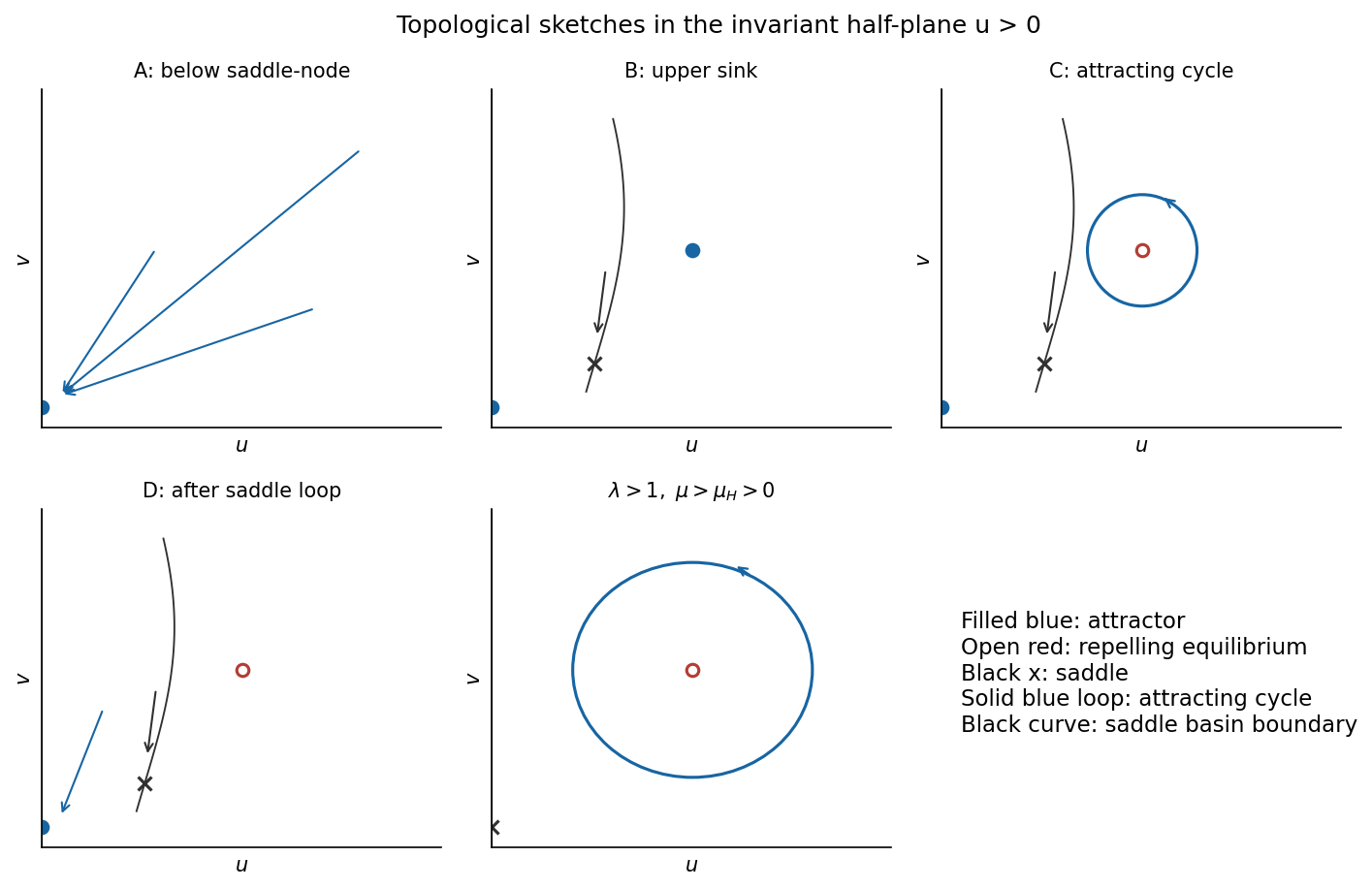
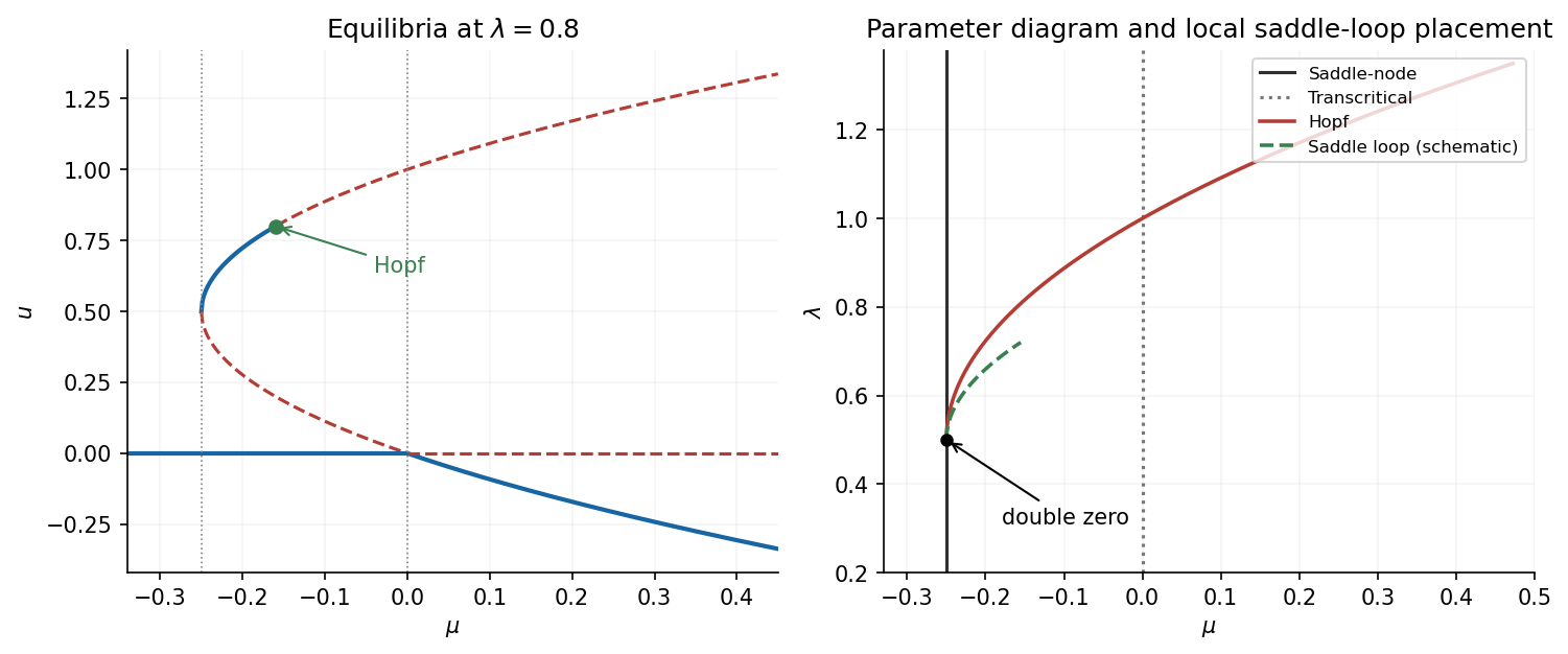
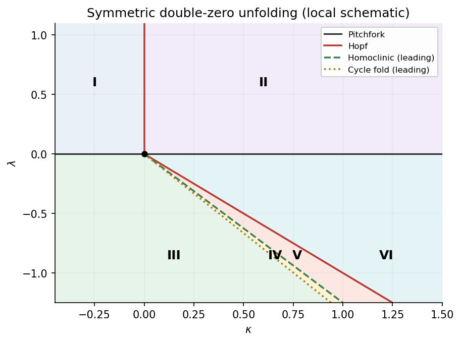
The no-cycle region D continues around the double-zero point onto the λ<1/2 side. The sketches distinguish the boundary origin from the two interior equilibria and show the periodic orbit only in region C.
The figure usesa representative λ>1/2; the upper branch's additional Hopf change is indicated. For λ<1/2 the upper branch is unstable everywhere on its existence interval. The exact trace criterion in part (a) specifies stability for every fixed positive λ.
The two nonzero branches exist for μ≥−1/4, coincide at equality, and the lower branch coincides with the origin at μ=0. For −1/4<μ<0 both are in u>0; for μ>0, P− has u<0 and P+ has u>0.
At the origin, the eigenvalues are μ,−λ. At any nonzero equilibrium(s,s2), using μ=s2−s gives
At H=0, B=4/5. The derivative of the denominator diverges positively there, while that of the numerator stays finite, so B initially decreases. Rescaling at large H gives B(H)∝H, so it eventually increases. At its minimum the stable and unstable selected periodic orbits meet. Thus the outer-cycle fold in a weakly perturbed double-well oscillator has κfold=cf(−λ)+o(∣λ∣) with 0<cf<4/5; quadrature gives cf≃0.75226. The decreasing portion of B(H) selects the unstable periodic orbit, and the increasing portion selects the stable one, since the energy drift has sign β−B(H).
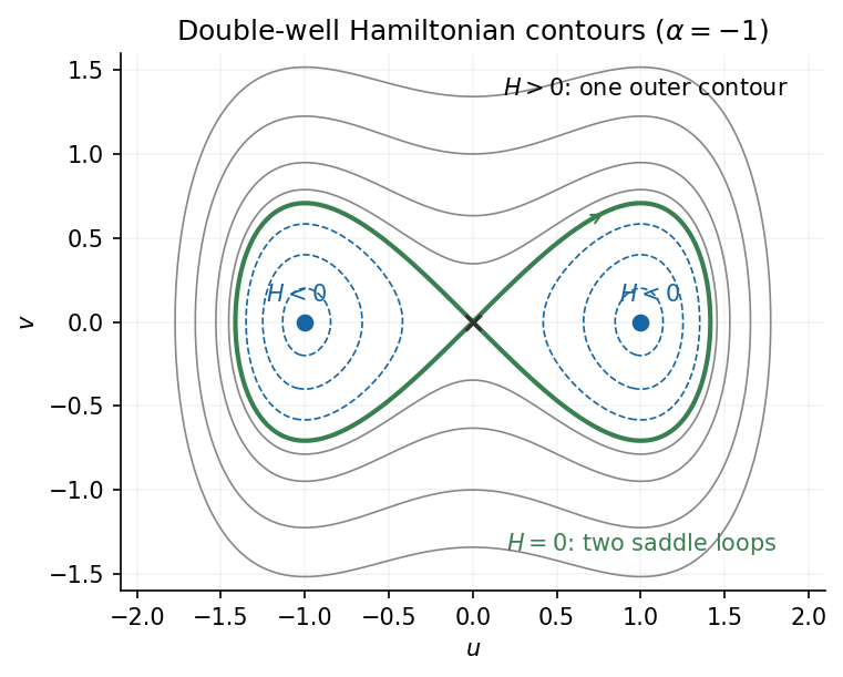
For α=−a02<0, the potential is a double well. Its minima are at u=±a0, where H=−a04/4; these are centre equilibria. The origin is a saddle equilibrium and has H=0. Energies −a04/4<H<0 give two separate closed contours, one in each well. Energies H>0 give a single closed contour surrounding both wells. The intervening figure-eight consists of two homoclinic loops:
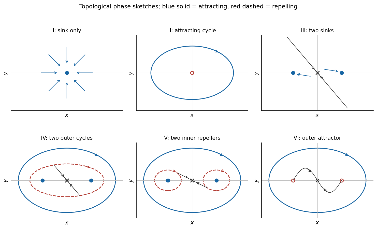
For κ=0 on the pitchfork curve, a leading centre-manifoldequation is x˙=(λx+x3)/κ+⋯. For κ<0, with unfolding parameter −λ, the pitchfork is supercritical and creates two sink equilibria from a sink equilibrium that becomes a saddle equilibrium. For κ>0 it is subcritical in the centre direction; the nonzero branches are unstable, and the transverse eigenvalue is also positive. The origin of parameter space is a reflection-symmetric double-zero degeneration.
To determine Hopf criticality at the origin, use the energyE=y2/2+λx2/2+x4/4, whose derivative is (κ−x2)y2. For a small nearly harmonicoscillation x=Rcos(λt), averaging gives R˙=κR/2−R3/8+⋯. Thus this Hopf bifurcation is supercritical and creates an attracting periodic orbit for κ>0. By the supplied opposite-criticality fact, the simultaneous Hopf bifurcations at the two nonzero equilibria are subcritical. A direct calculation confirms this: writing x=−λ+X, Y=−y/−2λ puts the cubic radial coefficient at 1/4>0, including the contribution from the quadratic terms.
The figure includes these local curves and the global curves derived below. All lines emerging from the double-zero point are local asymptotic sketches.
If x>1/2, the axial component is instead a=(2xe(2x−1)t/τ1−1)/(2x−1) and grows exponentially without bound, while b→1/(1+x). At the boundary x=1/2, which lies between the two stated regimes, a=1+t/τ1 grows linearly and b→2/3.
Normalization makes the molecular orientation finite even when the unnormalized conformation tensor diverges. For 0≤x<1/2, direct division by a+2b gives
The same normalized limit holds at x=1/2, agreeing continuously with the limit of the subcritical expression. The limiting orientations have nonnegative eigenvalues and unit matrix trace, as required for the normalized molecular orientation.
Now set S(t)=B(t):K=s(a−b)/(a+2b). Its limiting value is
If S∞>1/τ2, the coefficient is eventually positive, and the positive stretch grows without bound. At equality a bounded stretch would imply λ˙→1/τ2>0, which contradicts boundedness. Thus equality is not an additional bounded steady regime.
The function S∞(s) is continuous and strictly increasing from zero to infinity. Consequently there is a unique critical extension rate defined by
and the molecular stretch remains bounded precisely for γ˙<γ˙c. This is distinct from the tensor threshold γ˙τ1=1/2. If τ2<2τ1, for example, the normalized orientation can remain well defined and the stretch remain bounded for some rates above the tensor threshold; divergence of A alone does not prove divergence of the physical stress.
Its zero-rate limit is Gτ1=3μ0, recovering the Trouton ratio of three. The restrictions exclude both loss of a finite tensorsteady state and loss of a finite stretch steady state; neither denominator may be continued through its singularityasa physical steady constitutive response.
Its matrix trace has no forcing, because incompressibility gives trK=0. Starting relaxed, tra=0. The first-order stretch equation is Dtℓ+ℓ/τ2=(I/3):K=0, hence ℓ=0. Consequently B=I/3+a/3+O(ε2), and its anisotropic stress is Ga/3. From the relaxed remote past,
Stretch first changes at second order. Its equation gives λ−1=τ1τ2tr(A12)/6+O(3). Multiplication by λ2 therefore adds only an isotropic stress at second order; multiplying its second-order increment by the anisotropic first-order term would be third order. Absorb these isotropic corrections into p∗ to obtain
Equivalently, in σ=−pI+μ0A1+α1A2+α2A12, the constants are α1=−Gτ12/3 and α2=2Gτ12/3. The general small-amplitude linear response above permits fast oscillation; the local second-order fluid expansion also requires the slow-flow ordering just used.
With its material state fixed by a prescribed deformation history, the differential pom-pom model is asimple-fluid constitutive law. The stress depends on the local history of a material element through its molecular stretch and orientation, without gradients of that history between neighbouring elements. A differential representation does not prevent a material from being a simple fluid.
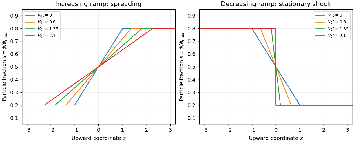
The transition widens linearly and its gradient decreases. At large time it approaches a rarefaction wave, with s≃(1+z/τ)/2 inside its expanding transition.
For the decreasing ramp, z=ξ(1−0.6τ) and the characteristic curves converge. Before they meet,
and the incoming characteristic speeds satisfy a(0.8)=0.6V0>0>a(0.2)=−0.6V0, which makes it an admissible entropy shock. The discontinuity transports no net excess particle flux because both plateau fluxes equal −0.16V0. These are local solutions before a finite container's boundaries affect the transition.
This formula gives the first characteristic crossing: minimize the positive values of −1/[f′′(s0)s0′]. At α=0 neither ramp changes shape; both move down at V0. For 0<α≤3/2, the flux is convex throughout 0.2≤s≤0.8: the increasing ramp spreads and the decreasing ramp steepens, although its entire ramp generally no longer focuses simultaneously. For α≥9, the flux is concave throughout that interval and these roles reverse. At the endpoint values the curvature vanishes at one plateau; it does not reverse sign inside the interval.
For 3/2<α<9, the inflection si=2/(α+1) lies between the plateau concentrations. Below si the increasing ramp spreads, while above it that ramp compresses; the decreasing ramp has the opposite local behavior. After characteristic crossing, the entropy solution can contain both a shock wave and a rarefaction wave. Quantitatively, an increasing step is selected by the lower convex envelope of f on the interval between its states: curved portions supply rarefaction waves, and straight portions supply shock waves. A decreasing step uses the upper concave envelope. A join between a fan and a shock wave at a state s∗ satisfies the tangent-chord relation f′(s∗)=[f(sb)−f(s∗)]/(sb−s∗), where sb is the other shock state. Thus curvature, not simply the magnitude of α, decides the wavepattern; the envelope may reduce to one shock if the tangent lies outside the state interval.
Welcome to the OurBigBook Project! Our goal is to create the perfect publishing platform for STEM subjects, and get university-level students to write the best free STEM tutorials ever.
Everyone is welcome to create an account and play with the site: ourbigbook.com/go/register. We belive that students themselves can write amazing tutorials, but teachers are welcome too. You can write about anything you want, it doesn't have to be STEM or even educational. Silly test content is very welcome and you won't be penalized in any way. Just keep it legal!
a Q&A website like Stack Overflow, where multiple people can give their views on a given topic, and the best ones are sorted by upvote. Except you don't need to wait for someone to ask first, and any topic goes, no matter how narrow or broad
This feature makes it possible for readers to find better explanations of any topic created by other writers. And it allows writers to create an explanation in a place that readers might actually find it.
This way you can be sure that even if OurBigBook.com were to go down one day (which we have no plans to do as it is quite cheap to host!), your content will still be perfectly readable asa static site.
 Codex 0 Created 2026-10-03 Updated 2026-10-14