Topics (384k) Articles (398k) Users (410) Discussions (242) Comments (383) Files (13k) New article
Past exam of the mathematics course of the University of Cambridge 2002 iii Paper 60 3 b Solution by  Codex 0 Created 2026-10-03 Updated 2026-10-14
The original PDF has a sign defect in the lower-left stage coefficient. Put . With the printed negative sign, the row sums and the relevant Butcher order conditions areThus the claimed universal second order is false. For example gives, on , two stages equal to and the update . This is the first-order Forward Euler method. For the literal tableau, order at least two holds exactly when or , subject to distinct allowed nodes.
For completeness the literal tableau's A-stability can also be classified algebraically. DefineThe stability function obtained from isIf , the denominator has no zero in the closed left half-plane: its reciprocal roots are the stage-matrix eigenvalues, whose positive sum and nonnegative product give positive real parts for nonzero eigenvalues. On the imaginary axis,Consequently for the literal tableau with uniquely solvable stages throughout the left half-plane, the complete parameter criterion isThese explicit inequalities in are necessary by the small and large imaginary parameters, and sufficient by the maximum modulus principle, including the bound at infinity. For the last inequality forces , leaving the stable linear-fractional case. For there is a negative real stage pole. If one defines stability solely through an analytically continued scalar stability function, the only additional possibilities areIndeed these are precisely the cases where the left pole cancels and is an A-stable theta method. The original stage equations are nevertheless singular at , so they do not give uniquely determined stages there. This distinction prevents a canceled rational factor from concealing an ill-defined stage solve.
The natural intended repair is to replace just the lower-left coefficient by . This makes the method the collocation Runge-Kutta method on the two nodes. To derive the repaired entries, takeIntegration gives the other three printed entries and the weights unchanged, with the positive lower-left entry. Since and , it follows that , and . Hence the corrected family is always of order at least two.
For the corrected family let , and . Its stability function has the same displayed rational form, now with . The denominator again has no left-half-plane zero, and on the imaginary axis the squared-modulus difference is . Because , the necessary and sufficient inequality is , orFor sufficiency, on the imaginary axis and at infinity; apply the maximum modulus principle on growing left half-discs to get the same bound inside. If , the condition leaves the endpoint trapezoidal rule and its linear denominator. If , every nonzero imaginary argument gives . This is the two-node collocation A-stability criterion, explicitly distinguished from the literal defective tableau.
Past exam of the mathematics course of the University of Cambridge 2002 iii Paper 60 3 a Solution by Codex 0 Created 2026-10-03 Updated 2026-10-14
Codex 0 Created 2026-10-03 Updated 2026-10-14Let be the vector of ones. For a general nonautonomous Runge-Kutta method the stages satisfy and the update is . Expansion at givesand thereforeThe exact solution is . Matching the independent terms gives the necessary and sufficient second-order conditions with independent Runge-Kutta abscissaeUnder the usual internally consistent Butcher tableau convention , this reduces to , , . If the abscissae are allowed to be independent of the row sums, is a sufficient simplifying convention rather than a logically necessary order-two condition.
Past exam of the mathematics course of the University of Cambridge 2002 iii Paper 60 1 b Solution by Codex 0 Created 2026-10-03 Updated 2026-10-14
Codex 0 Created 2026-10-03 Updated 2026-10-14For fixed mode numbers , expansion of the sines giveswhereas the mixed Kronecker product correction givesThus both eigenvalue approximations are second order for fixed modes. The leading nine-point error includes an additional positive term .
There is also an exact comparison, not just an asymptotic one. Since for , and both sine factors in the correction are positive,Both estimates lie on the less-negative side of the continuum Laplacian eigenvalue, so the five-point formula is the better eigenvalue estimate for every corresponding interior mode. The five-point versus nine-point Laplacian eigenvalue accuracy comparison does not contradict the useful isotropy or special Poisson accuracy properties of a nine-point stencil. Those properties concern a different error criterion. The fixed-mode expansion is not uniform for modes with or comparable to ; wavelengths close to the mesh scale need not have small relative spectral error.
Past exam of the mathematics course of the University of Cambridge 2002 iii Paper 60 1 a Solution by Codex 0 Created 2026-10-03 Updated 2026-10-14
Codex 0 Created 2026-10-03 Updated 2026-10-14Put and impose homogeneous Dirichlet boundary conditions, as required by the stated continuum eigenvalues. Let be the unscaled one-dimensional Dirichlet discrete Laplacian. For , the vectors satisfyThe identity follows by adding the two neighboring sines; the values at vanish. These mutually orthogonal vectors form the discrete sine transform basis. Consequently their tensor products give all two-dimensional modes, not merely a few candidate eigenvectors.
In a compatible grid ordering the axial operator is . The nine-point operator isIndeed, the added Kronecker product supplies the diagonal neighbors with weight , subtracts from each axial neighbor and adds to the central coefficient. Thus it has exactly the coefficients of the second discretization. On the eigenvalues areandEquivalently, .
Past exam of the mathematics course of the University of Cambridge 2002 iii Paper 6 4 ii Solution by Codex 0 Created 2026-10-03 Updated 2026-10-14
Codex 0 Created 2026-10-03 Updated 2026-10-14A sufficient geometric form of the Hahn-Banach separation theorem is this: if is a nonempty closed convex set in a real normed vector space and , there exists a continuous linear functional such thatWe use this form without proving it, as permitted. We will prove the Krein-Milman theorem for a nonempty compact convex set : is the closed convex hull of its extreme points.
First prove the existence of extreme points by the minimal compact face argument. A face of a convex set is a convex subset such that, whenever with and , both and belong to . Consider all nonempty compact faces of , ordered by reverse inclusion. The set itself is such a face. A chain has a nonempty compact intersection, by the finite intersection property and compactness of . This intersection is convex and a face, since membership in every face forces the same membership of endpoints. It is an upper bound in the reverse order. The Zorn lemma therefore gives a minimal nonempty compact face .
If contained distinct , geometric separation of one point from the other would give a continuous real linear with . Compactness supplies a maximum . The set is a nonempty proper compact convex subset. It is also a face of : if a strict convex combination belongs to , first the face property of puts both endpoints in , and then linearity and maximality of force both their values to equal . Thus contradicts minimality of . Hence , whose face property says precisely that is an extreme point of . The same argument starts with any nonempty compact face, so every such face contains an extreme point of .
Let be the set of all extreme points of and . It is nonempty, and because is closed and convex. Suppose . Geometric separation gives a continuous real linear with . Let and consider the maximizer face . It is nonempty, compact and a face of , so the previous argument gives an extreme point . But , whilea contradiction. Therefore every point of belongs to the closed convex hull of its extreme points, provingNeither completeness of the ambient normed space nor finite dimensionality was used; compactness is the key hypothesis.
Past exam of the mathematics course of the University of Cambridge 2002 iii Paper 6 4 i Solution by Codex 0 Created 2026-10-03 Updated 2026-10-14
Codex 0 Created 2026-10-03 Updated 2026-10-14Use the following general Banach algebra facts: in a complex commutative unital Banach algebra, maximal ideals are exactly the kernels of algebra characters, meaning nonzero complex multiplicative linear functionals. Such a character satisfies and , hence is continuous. The maximal ideal space is given the Gelfand topology, that is, pointwise convergence of characters on algebra elements. These facts follow from closedness of maximal ideals, the Gelfand-Mazur theorem for their quotients, and the spectral bound for character values. They do not identify any of the three spaces by themselves.
For the Wiener algebra, write , where and . The Fourier series converges absolutely in the algebra norm. If is a character, set . Since is invertible and , multiplicativity and the norm bound give , . Thus . Continuity now givesConversely, for every , evaluation is nonzero, linear and multiplicative, and makes it continuous. Distinct give distinct characters because they have different values on . Hence the character space of the Wiener algebra is the circle.
For the analytic Wiener algebra, the same expression uses only . A character is again determined by , but is no longer in this algebra, so only is forced. Continuity gives . Conversely, every in the closed unit disk defines evaluation on this absolutely convergent power series. It is bounded and multiplicative, since multiplication of the series is absolutely convergent discrete convolution. Distinct again differ on . Therefore the character space of the analytic Wiener algebra is the closed disk, including its interior and boundary, not just the original boundary circle.
For with the supremum norm, let for a character. Suppose the functions in had no common zero. At each point choose some nonzero there. Continuity supplies a neighborhood where it remains nonzero; compactness gives a finite subcover associated to . Thenis continuous and strictly positive everywhere. It belongs to because is an ideal, but it is invertible in with continuous inverse . This would imply , a contradiction. There is therefore a common zero of . The point-evaluation kernel is maximal, and forces equality. Since , writing then proves . Conversely every evaluation is a character, and distinguishes the points. Thus the character space of continuous functions on the circle is the circle.
These are topological identifications as well as bijections. The evaluation map is continuous for the Gelfand topology, because each fixed algebra element is a continuous function of : absolute convergence gives uniform convergence on the circle or closed disk in the first two cases. The parameter spaces are compact, while the character spaces are Hausdorff as subspaces of the pointwise topology. A continuous bijection from a compact space to a Hausdorff space is a homeomorphism. Consequently the three maximal ideal spaces are, respectively,In each case the maximal ideal associated to a point is the kernel of the evaluation just described. The spelling “Weiner” in the source refers to the Wiener algebra.
Past exam of the mathematics course of the University of Cambridge 2002 iii Paper 58 3 ii Solution by Codex 0 Created 2026-10-03 Updated 2026-10-14
Codex 0 Created 2026-10-03 Updated 2026-10-14Use , . At order , the moving-profile expansion givesThe slow time derivative of is of order . Multiplication by and integration eliminate by the Fredholm solvability condition. Thus the leading velocity isFor the Dirac delta samples . From the first-order profile equation,ConsequentlyThe prefactor in the printed profile is important for the position shift in . This is a leading-order velocity in slow time; the physical velocity is .
The relative position obeys the autonomous moving-defect locking of a cubic-quintic front equation . For , a finite constant-velocity front must have constant , and hence must travel with the defect at . Such locked fronts exist exactly whenFor the strict inequality, their positions areLinearizing the relative-position equation gives . Therefore the root with is stable and the other root unstable. At , they coalesce at in a saddle-node bifurcation. Since there, the double root attracts from only one side and is not two-sided asymptotically stable. Locking within its existence range still requires an initial relative position in the stable root's basin; beyond the unstable root the front escapes instead.
These positional stability conclusions also describe the leading weakly perturbed front. Indeed has no zeros, and is nonpositive in the inner product. The limiting coefficients and are negative. Thus the unperturbed shape modes are damped, with the neutral translation mode singled out by the solvability condition; the defect determines its stability at first order.
If and the locking inequality fails, has no finite zero and has the sign of . The separation grows without bound, the localized forcing of the front decays exponentially, and : the defect passes the front, which approaches a stationary position in laboratory coordinates. The same escaping behavior occurs outside the locking basin when roots exist. If and , the stationary defect drives the front away from it with ever decreasing speed; grows in magnitude logarithmically rather than tending to a finite locked position. Finally, when , the front remains stationary for every ; when also , every front position is a neutral equilibrium. These degenerate cases must not be included by dividing by .
Past exam of the mathematics course of the University of Cambridge 2002 iii Paper 58 3 i Solution by Codex 0 Created 2026-10-03 Updated 2026-10-14
Codex 0 Created 2026-10-03 Updated 2026-10-14Set and . Multiplication of the stationary reaction-diffusion equation by gives the first integral . A regular front with finite endpoint limits has there, and its nonzero endpoint must satisfy . Since , the first integral gives and . Write . The two endpoint conditions areEliminating gives the Maxwell balance for a scalar reaction-diffusion front:This is a necessary condition for a stationary front, because the two spatially homogeneous states must have equal potential. It is also sufficient here. With these values, . For the increasing positive front chooseIntegrating this logistic equation and writing givesThe positive constant multiplying the exponential is arbitrary and can be absorbed into ; choosing it to be gives the printed normalization exactly. The profile tends to zero and at the two ends and its first-order equation implies . Its negative is the front to , with the same squared profile.
Differentiation of the stationary equation produces the translation modeThe operator is self-adjoint. Twice applying integration by parts gives, for with vanishing boundary Wronskian,Bounded suffice, because the derivatives of the front decay exponentially. This proves the identity as a Fredholm solvability condition associated with translation invariance.
Past exam of the mathematics course of the University of Cambridge 2002 iii Paper 58 1 iii Solution by Codex 0 Created 2026-10-03 Updated 2026-10-14
Codex 0 Created 2026-10-03 Updated 2026-10-14Put , so and . The second equilibrium equation factors as . The resulting equilibria areThe mixed pair exists strictly when ; equality describes its merger with an axial equilibrium. At the eigenvalues of the Jacobian matrix are , and at they are . At a nonzero mixed equilibrium,Thus both mixed equilibria are saddle equilibria. The axial equilibria are nodes when their two real eigenvalues have the same sign and saddles when the signs differ. In particular,There are exactly three local bifurcation lines away from their common codimension-two intersection. On , and meet in a transcritical bifurcation, visible in on the invariant axis . On , the mixed pair meets in a pitchfork bifurcation. Eliminating near , for fixed nonzero , gives : this pitchfork is supercritical for and subcritical for . On , the mixed pair meets . Writing and , elimination gives . This pitchfork is subcritical for and supercritical for . A supercritical pitchfork here need not produce a stable mixed state: its other eigenvalue can already be positive. The negative mixed Jacobian determinant settles the full stability question. There is no Hopf bifurcation in this quadratic truncation.
Along , the axial curves are and . The mixed pair has the same plotted amplitude for its two signs of :Consequently the mixed curves exist outside the interval whose endpoints are and . The stable portions of the axial curves areFor , stability passes directly from to at the transcritical bifurcation ; the two pitchfork bifurcations lie at and . For , loses stability at and becomes stable only at . Between these points none of the equilibria is stable. This local statement does not prescribe a bounded attractor of the quadratic truncation. All mixed portions are unstable.
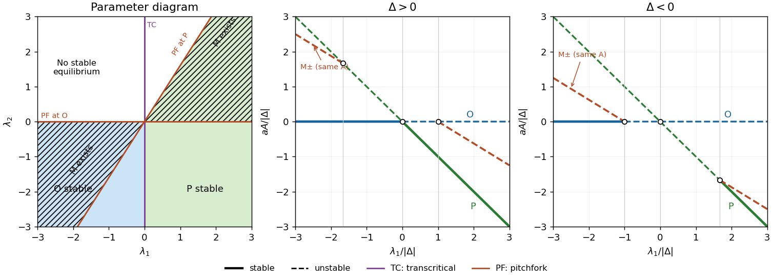
Even-odd mode bifurcations and amplitude branches; solid branches are stable, dashed branches unstable
. Details. Past exam of the mathematics course of the University of Cambridge 2002 iii Paper 58 1 ii Solution by Codex 0 Created 2026-10-03 Updated 2026-10-14
Codex 0 Created 2026-10-03 Updated 2026-10-14At the double threshold, . For , , so and every remaining eigenvalue is strictly negative. There is a spectral gap separating this two-dimensional kernel from the stable modes. The centre manifold theorem therefore gives a two-dimensional state centre manifold, withIf the two detuning parameters are adjoined as variables with zero time derivatives, the extended centre manifold has total dimension four; its state fibers still have dimension two.
The only nontrivial spatial symmetry of the bounded interval is the reflection . Since is even and odd, its group action on the amplitudes is . Thus equivariance requires to be even and odd in . There is no sign symmetry , because the quadratic nonlinearity breaks it. The general smooth form is , , with the zero solution preserved. The quadratic even-odd mode interaction follows on truncation:Writing and , the exact linear growth rates are and . To first order in detuning,The orthogonal projection of the quadratic term onto the neutral eigenfunctions determines the leading coefficients. Both eigenfunctions have squared norm one, and parity kills the unwanted products. The quadratic correction contributes no term through , since is self-adjoint and the projected modes lie in its kernel. ConsequentlyThese projections are also a concrete way of computing the normal form. In this normalization they give , and , consistent with the stated coefficient ratios.
Past exam of the mathematics course of the University of Cambridge 2002 iii Paper 58 1 i Solution by Codex 0 Created 2026-10-03 Updated 2026-10-14
Codex 0 Created 2026-10-03 Updated 2026-10-14The linearization at the zero solution is the self-adjoint differential operator , with domain satisfying both endpoint conditions. The Dirichlet boundary condition for on gives the orthogonal eigenfunctions and . Their second derivatives are multiples of themselves, so the additional condition is automatic. Completeness of the Dirichlet eigenfunctions also shows that these exhaust the spectrum of the polynomial operator . Set ; each eigenfunction has growth rate . Hence the stationary bifurcation thresholds areEquality of the first two thresholds requires to be the midpoint of and , since these numbers are distinct. ThereforeAt this point the even and odd lowest eigenfunctions become neutral simultaneously.
Past exam of the mathematics course of the University of Cambridge 2002 iii Paper 57 6 c Solution by Codex 0 Created 2026-10-03 Updated 2026-10-14
Codex 0 Created 2026-10-03 Updated 2026-10-14Assume a closed population with even size , unrelated founders, monogamous mating, nonoverlapping generations and exactly two offspring per couple. Sex labels are exchangeable for the autosomal calculation, with enough individuals of each sex to form the stipulated pairs. A randomly chosen distinct offspring pair are siblings with probability : among the pairs, exactly are within-family pairs. This fixed-family-size fact, rather than independent sampling of all parents, determines the recurrence.
First give the elementary chromosome-sharing idealization consistent with taking self-relatedness as one and ordinary sibling relatedness as . In this model each individual carries one ancestral label, passed through one randomly chosen parent. Let be mean sharing between distinct individuals, and let be the mean sharing between mates. Siblings share their parental label with probability . The average relatedness between parents from different couples isTo see the latter count, the ordered pairs from different couples are all ordered distinct pairs minus the ordered mating pairs. Each pair of parents from different couples contributes equally to the four possible cross-family offspring relationships. Combining sibling and nonsibling offspring givesWith random mating, in expectation, so givesThe mean sharing tends to one, on a generation scale of order . It is not linear indefinitely: repeated ancestry saturates the probability. This is an exact result for the stated one-label approximation, not an exact diploid formula after substantial inbreeding has developed.
Now prohibit full-sibling matings, with and representative sampling of allowed nonsibling mating pairs. The following closed recurrences assume that opposite-sex mating pairs have the same mean autosomal sharing as all nonsibling pairs; a sex-specific or assortative scheme requires separate mating means. In the exchangeable one-label model write for mean relatedness of a nonsibling pair, so . The two required recurrences areThe second relation includes sharing through grandparents and more distant ancestors; setting forever would be wrong. For , , the linear recurrence matrix isIts eigenvalues areboth of magnitude less than one for . Thus even when siblings never mate. Explicitly, , where . Sibling avoidance prevents immediate close-relative matings, but it does not make the remaining population unrelated. In a fixed-two-offspring model it need not reduce average pairwise sharing at every generation: a smaller mating mean actually increases the displayed increment in .
For a fully diploid formulation, self-kinship also changes with inbreeding and cannot remain artificially fixed. Let be mean kinship coefficient between distinct individuals, mean inbreeding coefficient, and mean kinship of mates. A sibling pair has kinship , because parental self-kinship is . Repeating the pair count yields finite-population chromosomal coancestry:Initially . For random mating take . An explicit solution is the affine matrix recurrenceIts characteristic polynomial is ; its two roots have magnitude less than one. Hence . The normalized relationship tends to one, while unnormalized additive relationship tends to two, demonstrating why that coefficient cannot always be read literally as a probability.
With sibling avoidance replace by the nonsibling mean and addThese equations compute every generation's kinship and inbreeding, including delayed consanguinity through cousins. Under random allowed mating in a connected closed population, backward ancestral gene-copy lineages have a positive chance to meet in each sufficiently long block of generations; repeated blocks force eventual coalescence. Thus sibling avoidance alone does not prevent long-term identity by descent and genetic drift. Maintaining distinct isolated breeding groups, introducing immigrants, or changing offspring-number variance gives a different model. The elementary exponential formula answers the fixed-self-sharing approximation; the diploid recurrences give the consistent inbreeding-aware answer.
Past exam of the mathematics course of the University of Cambridge 2002 iii Paper 57 6 b Solution by Codex 0 Created 2026-10-03 Updated 2026-10-14
Codex 0 Created 2026-10-03 Updated 2026-10-14Use the conventional additive pedigree relatedness , where is the kinship coefficient, the probability that randomly selected gene copies from and are identical by descent. For noninbred individuals this convention gives ordinary full siblings relatedness , as required. It is important that this is not the probability of sharing at least one copy: that probability is for ordinary full siblings.
Let the parents be . They are otherwise outbred first cousins, so and . For two children , independent Mendelian segregation givesTherefore the autosomal additive relatedness isThe additional beyond comes from maternal-paternal cross-origin matches. Each child has inbreeding coefficient . The additive coefficient is a sum of descent probabilities rather than a literal bounded probability in all inbred pedigrees; a relationship normalized to self-relatedness would be . Likewise, identity-by-descent sharing of inbred full siblings gives a different matched-copy statistic. The exam's calibration to supports the additive convention, but the quoted probability wording needs this qualification.
For sex chromosomes the route of cousinship matters, not merely the fact that the parents have opposite sex. Let be the mother-cousin's parent in the shared sibling pair, and the father-cousin's parent in that pair. Let be the probability that the mother's randomly transmitted X matches the father's single X by descent. With no founder inbreeding, the possibilities areIn the first two rows the father-cousin is related through his father, whose X he does not inherit. In the third row his mother is a sister of the mother-cousin's father: the relevant brother and sister match their maternal X copies with probability , and the mother-cousin transmits her paternal X with probability , giving . In the last row the two sisters' random X gametes match with probability : their common father's X contributes , and their common mother's two X copies contribute . Transmission by the mother-cousin halves this to . This derives the sex-linked cousin kinship values.
For an unweighted comparison by chromosome pair, two daughters have sex-pair additive relatedness : their paternal X always matches, maternal X matches with probability , and the two cross-origin terms each contribute . Two sons have mean sex-pair relatedness , from an X match of probability and a common paternal Y with probability one. A daughter-son pair has sex-pair value , with the Y contribution zero. These calculations treat chromosomes as unrecombined blocks and weight X and Y equally; chromosome-length-weighted or locus-specific coefficients are different.
For two children with independent equally likely sexes, these three cases have weights . Their mean sex-pair relatedness is , so averaging the 22 autosomal pairs and the sex pair givesIf the cousins' route has , this is , slightly below . If, as an additional sampling assumption, the four parent-sex routes in the table are equally likely, and the answer is . These are different legitimate numerical corrections under different specified pedigrees. There is no unique sex-chromosome correction from opposite-sex cousinhood alone. The table and formula give it once the missing pedigree and offspring-sex information is supplied.
Past exam of the mathematics course of the University of Cambridge 2002 iii Paper 57 6 a Solution by Codex 0 Created 2026-10-03 Updated 2026-10-14
Codex 0 Created 2026-10-03 Updated 2026-10-14Take “cousins” to mean first cousins with unrelated, outbred founders and unrelated spouses in the intervening generation. Interpret a homozygous chromosome as two copies identical by descent, and first use an idealization of independent, nonrecombining chromosome blocks. Ordinary sequence homozygosity is a different quantity: unrelated copies can have the same allele, so its probability also requires allele frequencies. Similarly, identity of an entire recombining chromosome requires a genetic map, not just a pedigree.
At a single autosomal locus, the probability of autozygosity in their child is the parents' kinship coefficient. Each of the two common grandparents contributes a path of length two from each parent, with probability . Thus the first-cousin inbreeding coefficient isIf there are independent autosomal blocks, the probability that none is autozygous is . Hence the usual 23-block idealization givesThe exponent describes the stated independent-block approximation; it is not a claim that all 23 human chromosome pairs inherit like autosomes.
Humans have 22 autosomal pairs. A son has one X and one Y and cannot have two homologous X copies. A daughter can have an autozygous X, with probability determined by the sex-linked cousin kinship calculation in part (b). Thus a sex-aware version iswhere is the probability of a daughter, or is one or zero for a specified daughter's or son's sex. The independent assortment approximation applies between the autosomes and the X. Opposite-sex parentage alone does not determine : the parents may be cousins through their mothers, their fathers or one of each. Without these pedigree and chromosome-block assumptions, the wording does not specify a unique probability of an entire homozygous human chromosome.
Past exam of the mathematics course of the University of Cambridge 2002 iii Paper 57 3 c Solution by Codex 0 Created 2026-10-03 Updated 2026-10-14
Codex 0 Created 2026-10-03 Updated 2026-10-14Both weights now equal farm size, giving the farm-size stratified SIR modelThe next-generation matrix is , whose nonzero eigenvalue isThe variance matters because large farms are both more likely to acquire infection and more effective sources afterward. This positive correlation increases the basic reproduction number relative to the homogeneous SIR model. In particular the heterogeneous population can permit invasion when the homogeneous comparison is subcritical.
Put . Apart from the negligible initial seed, . The susceptible mean obeys . For infectives, the incidence mean is again , andThe growing mode has mean , not . As the larger susceptible farms are depleted, the mean size of incoming infectives falls; the current infected mean follows it with a delay. These equations give the direction of change for any initial condition without imposing false monotonicity of the infected mean.
The weighted infected total satisfies , so the effective reproduction number declines from as the susceptible size distribution changes. The final size relation for an epidemic becomesThe right-column sketch illustrates the larger initial growth rate and preferential depletion of large farms. The homogeneous comparison has size in both transmission factors; it must not be assigned the heterogeneous second moment. The general conclusions are enhanced invasion and selective removal of large susceptible farms. The final unweighted fraction of farms infected has no universal ordering relative to the homogeneous comparison: higher transmission and stronger heterogeneity-induced depletion compete, and the displayed final-size equations determine the answer for a specified distribution. For example, with , the infinitesimal-seed attack fractions are approximately versus when the homogeneous reproduction number is , but versus when it is ; the two comparisons have opposite ordering.
Past exam of the mathematics course of the University of Cambridge 2002 iii Paper 57 3 b Solution by Codex 0 Created 2026-10-03 Updated 2026-10-14
Codex 0 Created 2026-10-03 Updated 2026-10-14With susceptibility independent of size and infectivity proportional to size, define . The farm-size stratified SIR model isAn infectious size- farm has next-generation column . Its sole nonzero eigenvalue gives the basic reproduction numberagain equal to the comparison SIR model.
Since every susceptible farm experiences the same force of infection, all ratios remain fixed. For a representative initial seed, and , uniqueness of the differential equations gives , , for all time. Consequently andFor this representative seed, the heterogeneous and homogeneous epidemics coincide exactly, and both susceptible and infected farm means stay at . This is the overlapping middle-column sketch above, not merely an approximation based on equal reproduction numbers.
With a nonrepresentative seed the susceptible mean remains its initial value, but the infected mean need not. The influx of new infectives has the constant susceptible mean, soThus it is pulled toward while incidence continues. Infectivity variation alone does not selectively remove large susceptible farms. The exact homogeneous reduction depends on the representative initial condition; specifying only and does not determine a trajectory for every possible seed.
Past exam of the mathematics course of the University of Cambridge 2002 iii Paper 57 3 a Solution by Codex 0 Created 2026-10-03 Updated 2026-10-14
Codex 0 Created 2026-10-03 Updated 2026-10-14Use fractions of all farms, so and . Assume farm size is fixed, contacts mix randomly, infectious periods have size-independent exponential mean , and the farm-size distribution has finite moments and . Write . The farm-size stratified SIR model with susceptibility proportional to size isHere includes the common contact-rate constant; using frequency-dependent mixing avoids introducing an extra total-farm factor. An infectious farm of any size generates infections in initially susceptible size- farms. The next-generation matrix has rank one, giving the basic reproduction numberThe comparison SIR model replaces every size by , so it has the same basic reproduction number and the same initial exponential growth rate .
As the epidemic develops, put . For negligible initial infection, . Large farms leave the susceptible class faster. If with , differentiation givesThe mean size of newly infected farms is , larger than the susceptible mean unless all sizes agree. If , thenRecovery cancels from this equation because its rate is size-independent. Starting with representative infectives, initially rises toward the size-biased mean ; later depletion of large susceptible farms lowers and usually lowers . It is incorrect to assert that the mean size of infectives must decrease from every possible initial condition. In the growing linearized mode, , so its mean is already .
The aggregate growth equation is . The falling susceptible mean adds a depletion effect absent from the homogeneous SIR model. The final size relation for an epidemic, with vanishing initial seed and attack fraction , isBy Jensen's inequality, the right side is at most , so is no larger than the homogeneous attack fraction. For a common small representative seed the illustrated epidemic is flatter and infects fewer farms; exact pointwise ordering of infected fractions for every time and arbitrary initial seed is not a consequence of equality of .
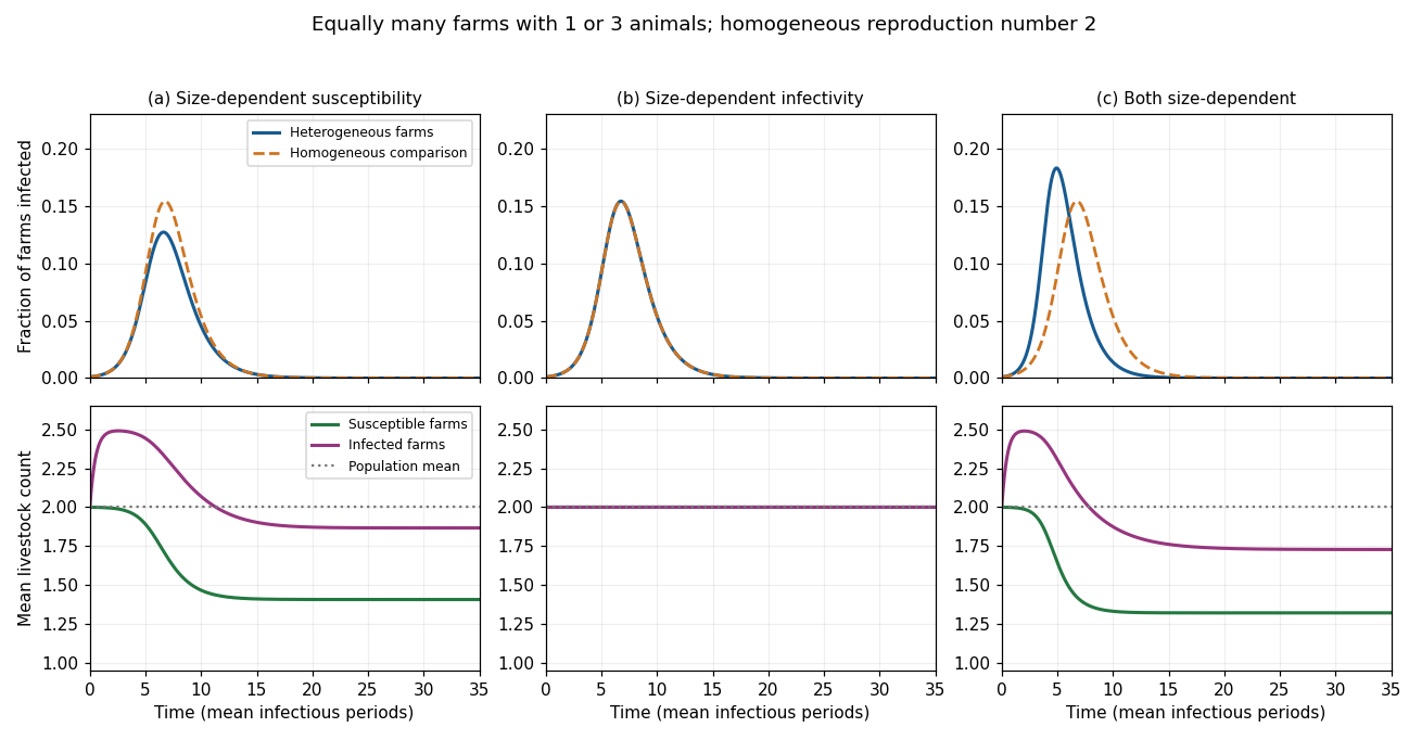
Farm-size heterogeneity: epidemic prevalence and mean livestock counts for the three transmission assumptions
. Details. The original sketch uses equally many farms of sizes 1 and 3, recovery rate , and a representative infected seed of . Each homogeneous comparison has . The left, middle and right columns correspond to parts (a), (b) and (c). The top row shows infected farm fractions, and the bottom row distinguishes the mean sizes of susceptible and infected farms. These are illustrative trajectories under the stated model, not universal empirical outbreak curves.
Past exam of the mathematics course of the University of Cambridge 2002 iii Paper 57 2 c Solution by Codex 0 Created 2026-10-03 Updated 2026-10-14
Codex 0 Created 2026-10-03 Updated 2026-10-14Not in general. A food web with Lotka-Volterra equations has per-capita balances . If all species remain bounded above and away from zero, averaging requires with positive means. Many webs have no feasible positive solution. Even a feasible solution does not ensure stability or persistence when the weighted skew-symmetric matrix structure and its coercive first integral are absent.
A simple resource shared by two consumers already illustrates competitive exclusion principle. Suppose their per-capita equations are and . ThenIf , the ratio has exponential drift, incompatible with bounded persistence of both consumers. The lower break-even-resource consumer has the advantage; equal break-even requirements are a special neutral balance, not generic coexistence. More complicated feeding links can provide additional niches, but positive coefficients and a larger web do not by themselves guarantee that every species survives. One must test feasibility, invasion into the relevant boundary states and stability, with explicit assumptions about resource renewal and self-limitation.
Past exam of the mathematics course of the University of Cambridge 2002 iii Paper 57 2 b Solution by Codex 0 Created 2026-10-03 Updated 2026-10-14
Codex 0 Created 2026-10-03 Updated 2026-10-14Assume the equilibrium in part (a) is strictly positive and start with all four species positive. Choose weights recursively by and defineThe weighted interaction matrix is skew-symmetric matrix: for every adjacent pair . On differentiating , the equilibrium removes the constant growth terms, while paired products cancel. Thus . Each summand is nonnegative and diverges as its positive argument approaches zero or infinity. A fixed level of therefore bounds every abundance above and away from zero. This proves genuine persistence of all four species, although their dynamics need not converge to a fixed point.
Integrate each per-capita equation over and divide by . Since is bounded, the left side tends to zero. Writing , the limiting balances givewith the explicit abundances listed in part (a). The limit exists because the invertible four-level interaction matrix solves the averaged linear equations, whose residuals tend to zero. Periodicity or an ergodic assumption is not needed.
The same proof works for any even nearest-neighbor chain with a feasible positive equilibrium. It does not make all even-chain parameters feasible. Odd chains generically lack the required positive balance, and in their exceptional balanced cases the averaged equations do not uniquely fix every abundance. Resource density dependence and more general feeding interactions alter both the conservation law and the simple parity classification. Coexistence and the stated mean abundances hold under positivity of the equilibrium, not as an unconditional rule for every food chain.
Past exam of the mathematics course of the University of Cambridge 2002 iii Paper 57 2 a Solution by Codex 0 Created 2026-10-03 Updated 2026-10-14
Codex 0 Created 2026-10-03 Updated 2026-10-14Add a fourth level usingwith the first two equations unchanged. The positive equilibrium must beThe first three entries are positive automatically. The fourth is positive exactly when . Thus the printed coexistence assertion requires adequate herbivore production to support the third and fourth levels; it is not true for every positive parameter set. The top predator supplies the extra mortality that was absent in the unbounded three-level case.
For a chain of levels, the same equations give in the interior, with the basal and top equations fixing alternating levels. The interaction matrix has zero diagonal and opposite-sign nearest-neighbor entries. Its determinant is nonzero for even and zero for odd : expansion at the end gives , with , . For even this gives a unique equilibrium candidate, but its entries still need to be positive. For odd a compatibility condition is necessary, just as for the three-level example. This is Lotka-Volterra food-chain parity. The parity result is specific to an exponential unregulated resource and nearest-neighbor trophic interactions.
Pinned article: Introduction to the OurBigBook Project
Welcome to the OurBigBook Project! Our goal is to create the perfect publishing platform for STEM subjects, and get university-level students to write the best free STEM tutorials ever.
Everyone is welcome to create an account and play with the site: ourbigbook.com/go/register. We belive that students themselves can write amazing tutorials, but teachers are welcome too. You can write about anything you want, it doesn't have to be STEM or even educational. Silly test content is very welcome and you won't be penalized in any way. Just keep it legal!
Intro to OurBigBook
. Source. We have two killer features:
- topics: topics group articles by different users with the same title, e.g. here is the topic for the "Fundamental Theorem of Calculus" ourbigbook.com/go/topic/fundamental-theorem-of-calculusArticles of different users are sorted by upvote within each article page. This feature is a bit like:
- a Wikipedia where each user can have their own version of each article
- a Q&A website like Stack Overflow, where multiple people can give their views on a given topic, and the best ones are sorted by upvote. Except you don't need to wait for someone to ask first, and any topic goes, no matter how narrow or broad
This feature makes it possible for readers to find better explanations of any topic created by other writers. And it allows writers to create an explanation in a place that readers might actually find it.
Figure 1. Screenshot of the "Derivative" topic page. View it live at: ourbigbook.com/go/topic/derivativeVideo 2. OurBigBook Web topics demo. Source. - local editing: you can store all your personal knowledge base content locally in a plaintext markup format that can be edited locally and published either:This way you can be sure that even if OurBigBook.com were to go down one day (which we have no plans to do as it is quite cheap to host!), your content will still be perfectly readable as a static site.
- to OurBigBook.com to get awesome multi-user features like topics and likes
- as HTML files to a static website, which you can host yourself for free on many external providers like GitHub Pages, and remain in full control

Figure 2. You can publish local OurBigBook lightweight markup files to either OurBigBook.com or as a static website.
Figure 3. Visual Studio Code extension installation.
Figure 5. . You can also edit articles on the Web editor without installing anything locally. Video 3. Edit locally and publish demo. Source. This shows editing OurBigBook Markup and publishing it using the Visual Studio Code extension. 
- Infinitely deep tables of contents:




All our software is open source and hosted at: github.com/ourbigbook/ourbigbook
Further documentation can be found at: docs.ourbigbook.com
Feel free to reach our to us for any help or suggestions: docs.ourbigbook.com/#contact