
Proper acceleration of a static Schwarzschild observer Created 2026-09-24 Updated 2026-09-24
A static observer at Schwarzschild radius must maintain the outward proper accelerationIt approaches the Newtonian value at large radius and diverges at the horizon.
Gravitational redshift between static Schwarzschild observers Created 2026-09-24 Updated 2026-10-14
For static observers at radii and , equal Schwarzschild-coordinate time intervals correspond to proper times . Hence
This static-observer relation is a special case of gravitational redshift, not a definition of every gravitational frequency shift.
Schwarzschild event horizon Created 2026-09-24 Updated 2026-10-03
The surface is the future event horizon of Schwarzschild spacetime. Its singularity in Schwarzschild coordinates is removable, whereas is a curvature singularity.
Schwarzschild tortoise coordinate Created 2026-09-24 Updated 2026-10-03
The tortoise coordinate satisfies
Schwarzschild radius Created 2026-09-24 Updated 2026-09-24
Equatorial null orbit in Schwarzschild spacetime Created 2026-09-24 Updated 2026-09-24
Radial Weyl curvature of Schwarzschild spacetime Created 2026-09-24 Updated 2026-09-24
With the curvature conventionthe vacuum Schwarzschild metric satisfiesThe opposite Riemann-sign convention reverses this sign.
Cosmological redshift Created 2026-09-24 Updated 2026-10-14
The cosmological redshift is the stretching of a freely propagating photon's wavelength between emission at cosmic time and reception at in an FLRW metric. For a comoving observer at each endpoint,Here are emitted and received wavelengths, and are the corresponding frequencies. A positive cosmological redshift means that the scale factor grew while the photon travelled. The name describes a shift toward longer wavelengths; it applies to light beyond the visible range as well.
For a computed example, let the scale factor double from to . An emitted wavelength of becomes , giving . The received frequency is half the emitted frequency. This determines a ratio of spatial rulers, not a recession speed: using as an actual velocity at is unjustified. The wavelength panel in the illustration under Hubble's law shows this doubling.
A short derivation follows successive wave crests along a radial null geodesic in FLRW spacetime. Their source and receiver have fixed comoving coordinates, so each crest traverses the same comoving distance:Shift both endpoint times to the next crest while keeping fixed. To first order in the very short periods , this gives . Locally, wavelength equals the speed of light times the crest period, yielding the displayed cosmological redshift relation. These periods are much shorter than the timescale on which the scale factor changes.
The relation isolates the smooth expansion contribution. An observed redshift can also contain a Doppler effect from source or observer peculiar velocity and a gravitational redshift. See combined kinematic and cosmological redshift for the multiplicative combination of endpoint motion and expansion. Treating every observed redshift as pure cosmological redshift can therefore misassign a nearby source's distance.
The useful insight is that a received wavelength ratio records how much the scale factor changed during the photon's journey. Turning that ratio into a distance requires an expansion history, through the Hubble parameter, and a specified convention such as luminosity distance or proper distance in cosmology; the ratio alone supplies neither.
Comoving coordinate Created 2026-09-24 Updated 2026-10-14
A comoving coordinate remains fixed for an observer following the homogeneous cosmological expansion.
A comoving coordinate provides labels for the comoving and proper distances comparison; proper separation additionally contains the cosmological scale factor.
Hubble parameter Created 2026-09-24 Updated 2026-10-14
The Hubble parameter is the instantaneous fractional rate of cosmic expansion:where the dot is a derivative with respect to cosmic time. Thus a short interval changes any fixed-comoving proper distance in cosmology by the fraction . Its dimensions are inverse time; describes expansion and contraction. The Hubble parameter identity gives .
RSA private exponent reveals the factorization Created 2026-09-24 Updated 2026-09-24
Knowledge of a valid public and private exponent gives , a nonzero multiple of . Writing it as with odd and testing random bases produces a nontrivial square root of one modulo with high probability; a greatest common divisor then factors . Thus one customer's private key under a shared semiprime modulus compromises every exponent using that modulus.
Common-modulus RSA attack Created 2026-09-24 Updated 2026-10-06
If the same invertible message is sent under one RSA modulus with coprime public exponents , choose integers with . From one recoversusing modular inverses for negative exponents.
Pitchfork bifurcation of a rotating hoop bead Created 2026-09-24 Updated 2026-09-24
At , the stable downward equilibrium of a rotating-hoop bead loses stability and two stable equilibria withemerge symmetrically.
Root-of-unity filter Created 2026-09-24 Updated 2026-09-29
For ,This is the finite geometric series identity and expresses orthogonality of the characters of .
Primitive root of unity Created 2026-09-24 Updated 2026-10-20
Equality case of the Heisenberg uncertainty relation Created 2026-09-24 Updated 2026-10-14
Equality in the Heisenberg uncertainty relation requires the centred vectors and to be imaginary scalar multiples, where , and are the expectation values. Thus, for some ,In the position representation, using the momentum operator turns this into a first-order differential equation, whose normalizable solutions areHence the quantum states saturating the Heisenberg uncertainty relation are these Gaussian wave packets, with arbitrary position and momentum means and global phase. Their width is . A Gaussian wave packet with an additional quadratic quantum phase need not saturate this product bound.
Quadratic-norm proof of the Heisenberg uncertainty relation Created 2026-09-24 Updated 2026-10-14
For an admissible quantum state with zero position and momentum means, positivity of the squared norm for every real givesThe discriminant is nonpositive, hence . Subtracting the expectation values from the position operator and momentum operator extends this outline to nonzero means.
Rolling without slipping Created 2026-09-24 Updated 2026-10-06
Rolling without slipping imposes that the contact point is instantaneously at rest, giving v=R omega.
Euler angles for a symmetric top Created 2026-09-24 Updated 2026-10-06
With the convention in which is inclination, is precession, and is body-axis spin, an axisymmetric body's kinetic energy is
Moment of inertia Created 2026-09-24 Updated 2026-10-14
The moment of inertia about a specified axis measures how a mass distribution resists changes of angular velocity about that axis. For point masses at perpendicular distances , or a continuous distribution with mass density ,Its SI unit is . The distance is to the entire axis, not to one point on it: moving a point mass along the axis leaves its contribution unchanged. The moment of inertia depends on both the distribution and the chosen axis; it is not determined by total mass alone. About an axis fixed in an inertial frame, a rigid body with larger moment of inertia has smaller angular acceleration under the same net axial torque, and greater rotational kinetic energy at the same angular speed.[ref]
For a simple model, put four equal point masses of total mass on light rigid spokes at radius . Their moment of inertia is . Doubling quadruples the moment of inertia without changing . The illustrated placements and give and . Actual spokes and finite-sized weights contribute their own moments of inertia; the point mass model neglects them. Repositioning weights during rotation also breaks the fixed-distribution assumption, so it requires a separate work and angular momentum calculation.
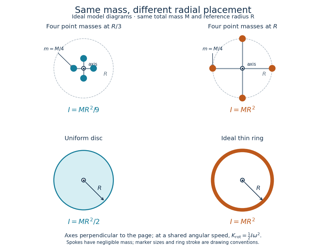
Same total mass, different radial placement and moment of inertia
. Original model diagrams, not experimental data. The upper pair has four equal point masses on negligible-mass spokes, at and from a perpendicular central axis. The lower pair compares a uniform disc with an ideal thin ring of the same mass and outer radius . The displayed moments of inertia determine rotational kinetic energy at a shared angular speed. The visible thickness of the ring and size of the point markers are only drawing conventions. Details.
The moment of inertia of a uniform disc follows by dividing it into concentric annuli: and . For an ideal thin ring every mass element is at , so . A ring of finite radial thickness instead uses the moment of inertia of a uniform annulus, , with inner radius . A moment of inertia is thus a compact summary of radial placement rather than a complete description of shape. For several joined pieces, their moments of inertia add only when each is calculated about the same axis.[ref]
A physical pendulum makes the moment of inertia measurable through timing. Martín Monteiro, Cecilia Stari, Cecilia Cabeza and Arturo C. Martí used a metal bar with suspension holes apart and an attached smartphone. They report bar length , bar mass and phone mass . Changing the suspension hole changes the pivot axis. Their readouts were phone gyroscope angular velocity records, analyzed by autocorrelation or a fit to a sinusoid, and an independent photogate; the logged records for the sinusoid fits lasted . They observed agreement between the three timing methods and the geometry-based model, including a minimum of oscillation period as the suspension point varied. These are reported apparatus details and observations, not measurements made for this article.[ref]
To infer a moment of inertia from such a measurement, determine the total mass including every attached part, locate the assembly's centre of mass , and measure its distance below the horizontal pivot . Record successive crossings in the same direction, or the elapsed time for complete oscillations, giving oscillation period . The physical pendulum model with a fixed pivot, a uniform gravitational field, negligible friction and the small-angle approximation givesThe crossing times, masses and geometric distances are the measured inputs; is an inference conditional on this model, while an integral over the assumed shape supplies an independent model prediction. The parallel axis theorem converts the inferred pivot moment of inertia to one about a parallel axis through . The controls and interpretation of that comparison are described there. An axial measurement determines one scalar moment of inertia, not the complete inertia tensor needed for general rotation.
There are unlisted articles, also show them or only show them.