
Möbius transformation Created 2026-09-24 Updated 2026-10-14
A Möbius transformation of the Riemann sphere has the formThe group is generated by translations, nonzero complex scalings, and inversion .
Projective quadric cone with one singular vertex Created 2026-09-24 Updated 2026-09-24
Over an algebraically closed field of characteristic other than two, the rank- quadricis an irreducible -dimensional cone for , and its singular locus is the omitted-coordinate vertex .
Affine cone over a projective hypersurface Created 2026-09-24 Updated 2026-10-03
If , its affine cone is . If is smooth, every nonzero point of is smooth; hence the vertex is the only possible singular point. The vertex is smooth for linear and singular whenever .
Pencil of plane curves Created 2026-09-24 Updated 2026-10-14
Given homogeneous polynomials of the same degree, their pencil is the one-parameter familyIts total space is the projective hypersurface , and projection to has these plane curves as its fibres.
Affine cone Created 2026-09-24 Updated 2026-09-28
For a projective algebraic set , its affine cone is the union in of the lines represented by the points of , together with the origin.
Averaged projected-gradient bound Created 2026-09-24 Updated 2026-09-28
If and , thenIt follows by expanding the squared distance after each projected step, using nonexpansiveness of projection, summing the resulting inequalities, and applying convexity.
Cylinder sigma-algebra Created 2026-09-24 Updated 2026-11-05
On a product space , the cylinder sigma-algebra is the smallest sigma-algebra making every coordinate projection measurable. Its generators ask finitely many coordinate questions. Every event in it depends on at most countably many coordinates: the collection of countably determined sets contains these generators and is closed under complements and countable unions. If is uncountable, the singleton consisting of the identically zero function is not such an event. Any countable coordinate test leaves an untested coordinate where a different function can be nonzero. Thus coordinate measurability alone need not capture every pathwise question.
Event Created 2026-09-24 Updated 2026-10-14
An event is a measurable set in a probability space: a question with a yes-or-no answer for each outcome. On , the event that the sum is at least nine consists of ten ordered pairs. Its probability is therefore under independent uniform dice. Saying that an event occurred means the actual outcome belongs to that set.
Lévy maximal inequality Created 2026-09-24 Updated 2026-11-05
Let be independent random variables taking values in a normed vector space, each symmetric in law: and have the same probability distribution. With partial sums , the Lévy maximal inequality isThe statement requires no finite moments. Symmetry is stronger than having zero expected value and is the key reflection hypothesis.
For a proof, let be the first crossing index. On , the future sum is independent of the past and symmetric. For any vector with , the two vectors and cannot both have norm at most : their average is , contradicting the triangle inequality. Symmetry therefore gives conditional terminal escape probability at least . Sum over the disjoint first-crossing events to obtain the inequality. This controls every intermediate partial sum using a single terminal tail.
Harris-FKG inequality Created 2026-09-24 Updated 2026-11-05
Concentration inequality Created 2026-09-24 Updated 2026-11-05
A concentration inequality bounds the probability that a random variable differs substantially from a typical value such as its expected value or median.
Second moment method Created 2026-09-24 Updated 2026-10-14
The second moment method uses a random variable's expected value and second moment to establish that a counted or measured quantity is positive with substantial probability. It is useful when a positive average alone could be caused by extremely large values on very rare outcomes. Controlling the variance rules out too much of that concentration in rare outcomes.
For a nonnegative random variable with and finite second moment, the second-moment bound for positivity givesEquivalently, . The method also includes the simpler Chebyshev's inequality bound . Thus a sequence of such random variables with has with probability tending to one. These statements require no independence assumption. The variance argument and its use for random counts are developed in Zhao's lecture notes. [ref].
For an original toy count, let count successes in ten independent Bernoulli trials with success probability . The binomial distribution givesConsequently . The exact probability is . The first moment method and union bound only give the upper bound here. First and second moments therefore answer complementary existence questions.
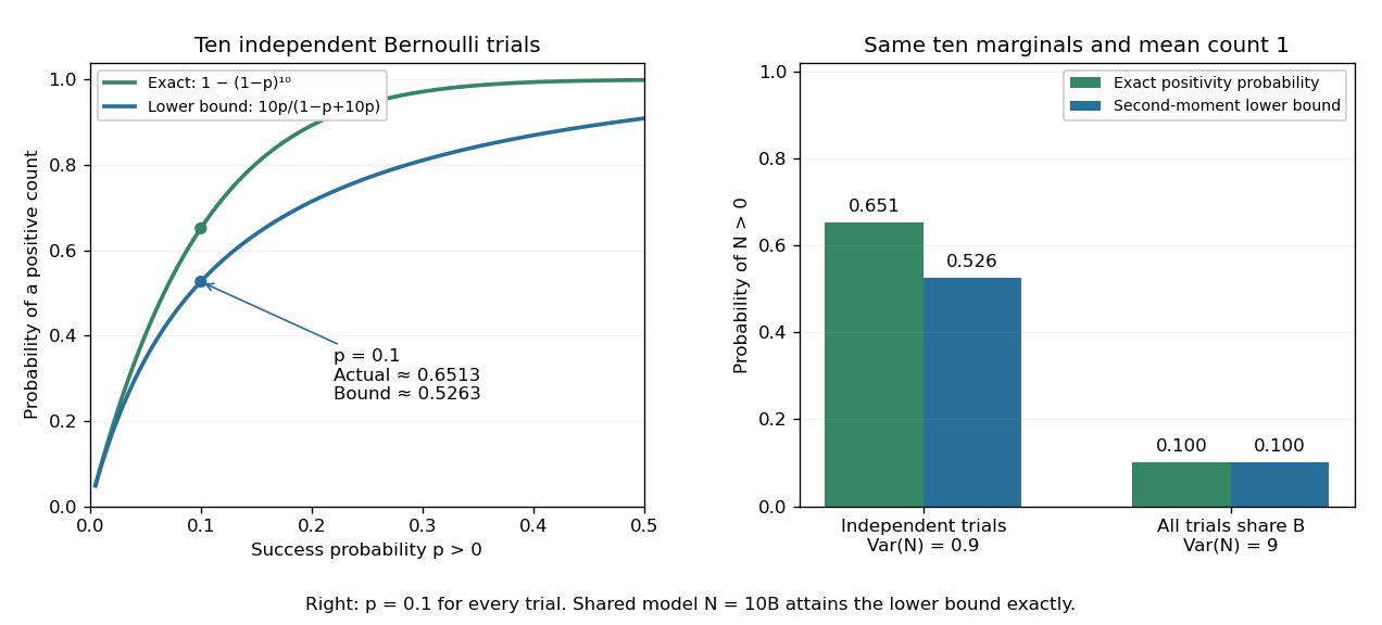
The second moment method certifies a positive count, while statistical dependence can change the conclusion despite an unchanged mean
. Left: exact binomial distribution probabilities of at least one success and second-moment lower bounds for ten independent trials as the success probability varies. Right: the same ten trials with either occur independently or share one common Bernoulli outcome. Both counts have mean one, but the perfectly linked count has much larger variance and only probability of being positive. All data are original specified probability models. Details.
For a sum of indicator random variables, the variance of a sum isIndependence makes the covariances vanish, but the formula itself also covers dependent counts. For the same ten success probabilities, let every trial share a single Bernoulli random variable : then , with mean one, variance nine, and . The second-moment lower bound is exactly . Ignoring the positive covariances would produce the false independent-count conclusion. Zhao's discussion of sums of indicators explains why overlapping counted structures require these pairwise terms. [ref]
https://ocw.mit.edu/courses/18-226-probabilistic-methods-in-combinatorics-fall-2022/mit18_226_f22_lec06-07.pdf. Zhao, MIT 18.226, §4.1: indicator covariances and Bernoulli counts
. First moment method Created 2026-09-24 Updated 2026-10-14
The first moment method uses the expected value of a count to control whether any counted occurrence exists. For a random variable taking nonnegative integer values, Markov's inequality givesConsequently, implies , proving that an outcome with no counted occurrence exists. For a sequence of such counts, shows that with probability tending to one. The first moment method uses information about the average count, while the complementary second moment method also uses its variance.
Exponential survival probability Created 2026-09-24 Updated 2026-11-05
Variance of a uniform distribution Created 2026-09-24 Updated 2026-11-05
Characteristic function of a uniform distribution Created 2026-09-24 Updated 2026-09-24
For uniform on , .
Weibull distribution Created 2026-09-24 Updated 2026-11-05
The two-parameter Weibull distribution is a positive lifetime model with shape and scale . Its Probability density function and Survival function areIts Cumulative distribution function is . The Hazard function is : it decreases for , is constant for , and increases for . This permits decreasing or increasing failure rates within one family.[ref]
The mean is and the variance is . The substitution reduces the power-moment integrals to gamma integrals. At the law is exponential with rate ; at its survival is .
Inverse transform sampling is explicit: for uniform on , take . Conditional survival after an already attained age is , which depends on unless . This is why an Unknown entry age in a Weibull survival segment affects the likelihood. The scale parameter here is ; inverse-scale parameterizations instead use its reciprocal.
Chi-squared distribution Created 2026-09-24 Updated 2026-11-05
A Chi-squared distribution with statistical degrees of freedom is a Gamma distribution with shape and rate . Its Probability density function isFor a positive integer , a variable is the sum of squares of independent standard normal random variables. The gamma definition extends the law to noninteger positive degrees of freedom; it does not require a fractional number of Gaussian coordinates.
Its mean is , its variance is , and its Moment-generating function is for . These follow directly from the Gamma density or by multiplying the squared-normal transforms in the integer case.
The law appears when Gaussian deviations are aggregated as a squared length. For iid observations with and , the Sample variance satisfies . Centering removes the one-dimensional sample-mean direction, leaving independent Gaussian coordinates after an orthogonal change of basis. This exact normal-sampling law underlies confidence intervals for a variance; it is not a universal variance-sampling formula for arbitrary data.
Normal distribution Created 2026-09-24 Updated 2026-10-14
The normal distribution is a probability distribution on the real line with mean and positive standard deviation . Its probability density function isIn the notation , the second parameter is the variance , not the standard deviation . The probability density function is symmetric about , highest there, and integrates to one. These formulas and the parameter convention are given in MIT 18.05, Reading 5c, §5: normal distributions.
The normal distribution is a location-scale family: if is a standard normal random variable, then . Changing moves the center; changing stretches the horizontal distances from it. The reciprocal factor lowers the probability density function as the curve widens, preserving total area. This is why one standard normal distribution suffices to calculate probabilities for the whole family. [ref].
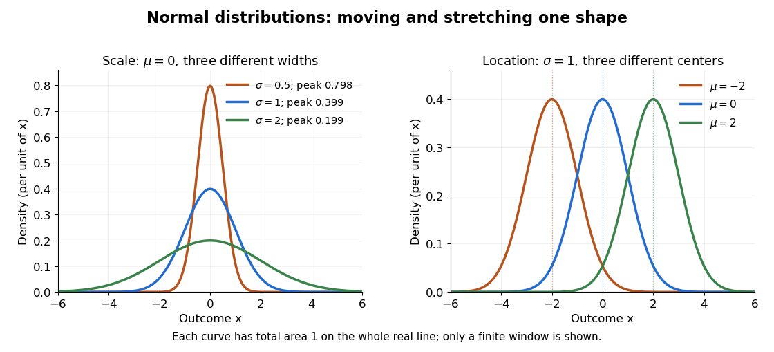

The height is a probability density function value, not . For , the probability is an area, and for every individual . If is measured in some unit, and use that unit, uses its square, and uses its reciprocal; the integral is a dimensionless quantity. A change of measurement unit therefore changes the height without changing the probability. The area interpretation is developed in MIT 18.05, Reading 5b: continuous random variables.
The usefulness of the normal distribution goes beyond its simple shape. Under the central limit theorem, sums of independent and identically distributed random variables with finite positive variance, after centering and scaling, approach the standard normal distribution. Thus approximations by a normal distribution can arise even when the individual random variables have quite different probability distributions. The hypotheses matter: a model of measurement error still needs evidence that this approximation is appropriate. [ref]
https://ocw.mit.edu/courses/18-05-introduction-to-probability-and-statistics-spring-2022/mit18_05_s22_class06-prep-b.pdf. MIT 18.05, Reading 6b, §5: standardization and the central limit theorem
. Exact closure under a linear combination of independent normal random variables provides another reason the family is convenient.Historically, the curve appeared in a different problem from fitting measurements. In the 1756 edition of The Doctrine of Chances, Abraham de Moivre reproduces work he dates to 12 November 1733 on approximating sums of binomial distribution probabilities for equally likely success and failure; page 245 already gives the one-sided central area as . [ref]
https://archive.org/details/doctrineofchance00moiv/page/243/mode/2up. De Moivre, The Doctrine of Chances, 1756, pp. 242–246
. In his 1809 Theoria motus, Carl Friedrich Gauss derived a normal distribution for measurement error from a condition on the arithmetic mean, then connected maximizing its likelihood to minimizing the sum of squared errors under that model, the principle behind ordinary least squares. These are distinct contributions: approximating binomial distribution probabilities and justifying an estimation rule. [ref]https://archive.org/details/theoryofmotionof00gausrich/page/258/mode/2up. Gauss, Theoria motus, 1809, §§177–179; Davis's 1857 English translation, pp. 258–260
.For a short normalization check, substitute in the integral of . The Gaussian integral gives , so the total area is one. The standard normal density is an even function, giving ; integration by parts gives . Then linearity of expectation and the variance scaling rule applied to yield mean and variance .
Joint distribution function Created 2026-09-24 Updated 2026-11-05
The joint distribution function of real random variables isIt determines probabilities of rectangles throughIts marginals are and similarly for . independence is equivalent to for every .
If the joint law has a Probability density function , then , and mixed differentiation recovers where justified. A joint density need not exist even when both marginals have densities. For example, take with uniform on . Writing for the uniform Cumulative distribution function gives . The law is concentrated on the diagonal , a set of two-dimensional Lebesgue measure zero. Its two uniform marginals therefore do not make it an absolutely continuous joint law.
There are unlisted articles, also show them or only show them.