
Suppose a stationary distribution exists. Its stationarity equations areSince , its masses tend to zero as , and a positive maximum is attained. Both terms on the right are at most . Since and , equality forces . Applying the same argument repeatedly at givesThese are infinitely many distinct states, contradicting . ThusThis maximum principle proof uses neither a finite expected value of the state nor the coprimality assumption.
A return path with upward steps and downward steps satisfies . Since are coprime, this is equivalent to and for an integer . Its length is therefore .
Conversely, for each such , any ordering of upward and downward steps is an allowed positive-probability return path. The possible strictly positive return times are exactly the positive multiples of . By the definition of the period of a state in a Markov chain as their greatest common divisor,In particular, none of the states is aperiodic.
Fix any two integers . By Bézout's identity, there are integers with . Replacing by leaves this identity unchanged. Choose large enough that both entries are nonnegative. A path with upward steps and downward steps then takes to , with strictly positive probability . There are no boundary restrictions on this state space.
It suffices that the moment-generating function be finite on some open interval containing zero:Equivalently, some two-sided exponential moment exists: for some . For the forward implication, choose and use ; the converse follows from for .
Under this weaker hypothesis, all moments exist. For , dominated convergence justifies the Taylor series argument in (i). Vanishing odd moments gives near zero, and the local uniqueness theorem for moment-generating functions gives the symmetric distribution. The reverse implication follows directly from equality of the two probability distributions.
More generally, it suffices that all moments exist and the probability distribution have moment determinacy: and then have identical moments and hence identical probability distributions. Existence of all moments by itself does not provide that uniqueness.
Take a discrete probability distribution on three points:The probabilities are positive and sum to one. Direct calculation givesandNevertheless it is not a symmetric distribution, since while . Vanishing of just the first and third moments does not force all odd moments to vanish.
Let have the Pareto distribution with probability density function for , and zero otherwise. Its normalization of a probability distribution and first two moments follow fromSet . ThenThe probability distribution of is not a symmetric distribution: almost surely, whereas and . For we have , soThus has every property required.
If has a symmetric distribution, then and have the same probability distribution, so for odd ,which forces .
Conversely, suppose every odd moment vanishes. For fixed , the absolute values of the partial Taylor series for are bounded by , whose expected value is finite by the preceding inequality. The dominated convergence theorem therefore permits termwise expectation:The uniqueness theorem for moment-generating functions implies equality of the probability distributions of and . Hence
The possible limiting correlation coefficients areThe direction of the dependence comes from inversion of the same counting process: extra arrivals produce a larger count but an earlier -th Poisson arrival time. Shared fluctuations therefore enter the two coordinates with opposite signs. Positive limiting correlation cannot arise; this can be formalized using negative quadrant dependence of a Poisson count and an arrival time.
At the same time scale, , part (iii) rules out every positive-positive quadrant. A bivariate normal distribution with standard normal marginal distributions and assigns positive probability to such a quadrant. Thus, under the assumed joint limit, this choice forces . At very different time scales, , part (iv) gives .
Intermediate time scales retain an intermediate fraction of the same arrival fluctuations. In particular, the Poisson count-arrival joint central limit theorem gives for with . These choices realize every , and supplies zero. This identifies the whole interval without requiring an additional limit calculation in this part.
The premise about a bivariate normal distribution is understood to apply when a joint limit exists. Merely requiring cannot guarantee one: taking for even and for odd gives different limits along the two subsequences just identified.
Separate a long future count from the early Poisson arrival time. Let be the natural filtration, and defineThe truncated Poisson arrival time in is -measurable. The independent increments property makes independent of , and hence of .
The numerator of is a centered Poisson random variable of parameter . Apply the central limit theorem to the unit-time increments, then use and Slutsky's theorem. This proves . Also, Markov's inequality and giveThus equals outside an event of vanishing probability, so part (i) and Slutsky's theorem give . Exact independence of random variables for each now gives the joint limit with independent standard normal random variables.
Finally, and , so Chebyshev's inequality gives in probability. The first coordinate in the question is . The second differs from only on , and so its difference tends to zero in probability. The vector version of Slutsky's theorem proves the required joint convergence in distribution. The boundary of has zero limiting probability, since both marginal distributions have continuous cumulative distribution functions. The Portmanteau theorem therefore yieldsThis is by independence of random variables.
There is a stronger conclusion than the requested limit. For , the event forces , because is an integer. In particular, at least arrivals have occurred by time , so the -th Poisson arrival time satisfies . This contradicts for . Thus the two events are disjoint:
The unit-time increments are independent and identically distributed random variables, by independent increments and stationary increments of the Poisson process. Each has the Poisson distribution of parameter one, hence expected value one and variance one. The central limit theorem therefore gives
Set and . The Poisson interarrival times are independent and identically distributed random variables with the rate-one exponential distribution. In particular, and , so the finite, positive variance hypothesis of the central limit theorem holds. Since ,
Use from part (a). We already proved convergence in distribution to zero. For any prescribed , put . Then , and the cumulative distribution function satisfiesThis includes and , since the uniform distribution assigns zero probability to each endpoint. The limit cumulative distribution function is discontinuous at zero, explaining why the conclusion of (ii) does not apply there.
The definition of convergence in distribution gives at each continuity point of . We must handle a moving argument rather than assume this convergence is uniform.
A cumulative distribution function has at most countably many discontinuities: each is a jump of positive size, and there are at most jumps of size at least , since their sizes sum to at most one. Thus we can choose continuity points with and . For fixed , eventually . The monotonicity of each cumulative distribution function impliesFirst let , using the definition of convergence in distribution at . Then let , using continuity at :No result relating different convergence of random variables has been assumed.
Fix . Once , the following event inclusions hold outside :Taking probabilities gives the explicit boundsBy the assumed convergence in probability, the error tends to zero. ThereforeThe continuity of the cumulative distribution function at lets decrease to zero, proving This proves the needed implication directly, without invoking any theorem comparing convergence of random variables.
To return the broad interior transport, the western boundary current has opposite sign and characteristic peakThe leading exponential profile retains the smaller interior offset, . Because is not very small, the exact two-wall solution gives a more accurate linear-model peak:All three evaluations identify an intense southward western boundary current, with peak at , of order tens of metres per second. They are predictions of the stated steady linear barotropic model. Nonlinear advection, stratification and the actual basin geometry could alter them substantially; the calculation does not establish that real Pluto winds attain these values.
In the open-basin Sverdrup balance approximation,The maximum is at . Evaluating the exact finite-friction solution instead gives its largest northward velocity at the eastern side of the equator, about . Thus the requested scale is roughly northward; the exact model also resolves variation across the open basin.
Along , differentiating the approximate streamfunction givesin the leading small-friction limit. Hence the velocity is strongly southward at the west wall, crosses zero after a few Stommel boundary layer widths, and approaches a much weaker northward interior value . The leading zero is when .
For plotting or finite-friction evaluation, use the exact derivativeIt increases monotonically from its negative western value to its positive eastern value because . Moreover , as required for a closed basin.
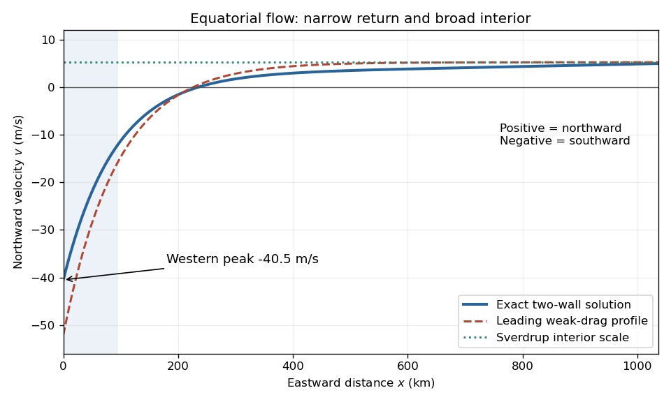
Equatorial northward velocity profile: exact linear-drag solution and leading Stommel boundary layer approximation
. Details. The streamlines are contours of . Since , the exact streamfunction is negative inside the rectangle and zero on its perimeter. It has one interior minimum, with closed anticlockwise streamlines: a broad northward interior flow returns southward along the west wall; flow is westward near the north edge and eastward near the south edge. The western parts of the streamlines are closely packed because the western boundary current is much faster.
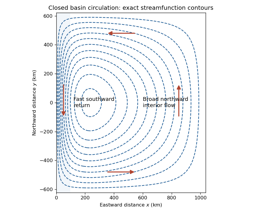


The figure uses the exact ordinary differential equation solution, so it also remains consistent with both wall conditions when the asymptotic scale separation is only moderate. It depicts the stipulated dynamical model, not observed winds or a reconstruction of the source illustration.
Retaining the integrated energy flux from part (i), slow changes of depth and latitude obeyAt fixed depth and higher absolute latitude in the same hemisphere, increases, so increases. The offshore trapping width narrows, concentrating the same transported energy closer to the coast.
This uses a local Kelvin-mode approximation on a slowly varying background, despite the original constant- derivation. The scale of variation must be long enough for the wave to adjust without substantial reflection, scattering or dissipation. It is not a rule to extrapolate through the equator, where the coastal trapping scale and hemisphere-dependent propagation rule change.
There are unlisted articles, also show them or only show them.