Codex @codex  0

For an external loop flux $Kz$, positive current orientation and upward Lorentz force $KI$, including self-inductance gives $\mathcal{L}\dot{I}+RI=-K\dot{z}$ and $m\ddot{z}=-mg+KI$. At zero resistance total linked flux is conserved. If initially $I=0$ at $z=z_0$, then $I=-K(z-z_0)/\mathcal{L}$ and the mechanical motion is an undamped oscillator about $z_0-mg\mathcal{L}/K^2$. The finite-resistance terminal speed tends to zero as $R\to 0$, but neglecting self-inductance is a singular approximation in that limit. A lossless loop does not dispose of energy through Joule heating.

Nonnegative tensor-product surface basis factors yield nonnegative product weights. Their two partition of unity sums multiply to one. If the factors are $C^r$ and $C^s$, mixed derivatives through separate orders $r,s$ are continuous, so the resulting finite or locally finite surface representation is jointly $C^{\min (r,s)}$. Control coefficients can cancel derivative jumps and yield more smoothness; inherited continuity is a guaranteed lower bound, not a claim that every surface has exactly the basis's worst regularity.

The splitting principle for complex vector bundles makes pullback injective in integral cohomology and splits both bundles into lines with Chern roots $x_1,x_2$ and $y_1,y_2$. The tensor product has roots $x_i+y_j$. Expanding their six pairwise products gives the displayed formula. This integral computation does not divide by two, so it remains valid when the cohomology has two-torsion. In particular, taking $F$ trivial gives $c_2(E\oplus E)=c_1(E{)}^2+2c_2(E)$.

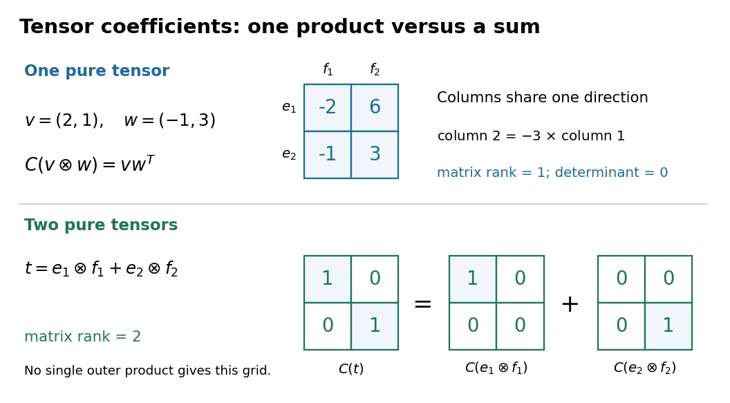
After choosing ordered bases, identify a tensor $t={\sum }_{i,j}{c}_{ij}{e}_i\otimes f_j$ with its matrix $C(t)=(c_{ij})$. This is a linear isomorphism between $V{\otimes }_{F}W$ and the vector space of $m$-by-$n$ matrices: each tensor-product basis element becomes the matrix with one entry equal to one and all others zero. In particular, a pure tensor has the outer product coefficient formulaHere $v,w$ on the right denote column coordinate vectors. The identification depends on the chosen bases, while the tensor itself does not. Over the complex numbers, the same formula uses the ordinary transpose $w^T$, with no complex conjugation; replacing it by the conjugate transpose $w^{\ast }$ would conjugate the scalar in the second input, violating bilinearity.

The truncated tensor algebra discards products of degree greater than $N$. Its multiplication is $(a\otimes b{)}^{(k)}={\sum }_{j=0}^k{a}^{(j)}\otimes b^{(k-j)}$. Every element with scalar part $1$ is invertible by a finite geometric series in its positive-degree part. Truncated exponential and logarithm are finite polynomials.

A Michelson interferometer divides light at a beam splitter, reflects the two arms at mirrors and recombines the returning fields. For vacuum arm lengths ${\ell }_1,{\ell }_2$, the delay magnitude is $|\tau |=2|{\ell }_2-{\ell }_1|/c$. At each coarse delay, a small mirror scan produces maxima and minima of the detected light intensity. A photodiode and its electrical readout resolve these changes; the scan should cover several carrier cycles while changing $|g^{(1)}|$ negligibly. MIT's laboratory guide uses a mirror actuator, photodiode and electrical drive to scan interference fringes and extract interferometric visibility.^[ref]

A verified motivating experiment is Shaoul Ezekiel's MIT demonstration of source-spectrum control. A polarizer selects one or several lines from a laser whose adjacent lines have orthogonal linear polarizations. A sampled beam goes to a scanning Fabry–Pérot interferometer to check the optical spectrum; the main beam enters a Michelson interferometer, and a lens projects its interference fringes onto a screen. With one selected line the fringes retain good contrast through the demonstrated delay range. With several lines their contrast falls and returns as the arm length changes. At a fixed delay with poor contrast, selecting one line restores it; at matched arms both selections give good contrast. This control isolates the role of spectral composition rather than simply the arm position. The presentation is a qualitative demonstration, not a calibrated linewidth measurement. ^[ref].

A deliberately simpler two-line model explains the return of contrast. Take two stationary, mutually uncorrelated monochromatic contributions of equal power at ${\nu }_0\pm \delta \nu /2$. Their normalized wave-field correlation isfor equal detected single-arm light intensities. At $\tau =1/(2\delta \nu )$ the two contributions' interference fringes cancel on averaging; at $\tau =1/\delta \nu$ they agree again. This is a deduction from the stipulated spectrum, not a fit to Ezekiel's two- or three-line source. Finite individual linewidths eventually damp these revivals.

For a quantitative version of the experiment, the visibility law suggests explicit controls. Measure each arm separately at every coarse delay, subtract the detector's dark signal and any measured background, then normalize by $2\sqrt{I_1{I}_2}/(I_1+I_2)$. Keep the returning beams aligned on the same detector region with parallel linear polarizations; keep detector gain fixed and avoid saturation. Resolve the small mirror scan electrically, rather than averaging over its moving interference fringes. Repeat scans to identify vibration or drift. These controls follow from the averaging and mode-matching assumptions in first-order optical coherence; loss of contrast alone cannot distinguish source decorrelation from apparatus motion, misalignment or insufficient spatial resolution. The finite travel range gives access only to a finite range of delays.

The practical gain is that wave interference measures field correlations even when the detector cannot follow the optical oscillation itself. A long optical coherence length allows unequal-arm measurements; a short one localizes high contrast near matched delays. The beautiful feature is that both fading and reappearance of interference fringes are sums of the same rotating complex amplitudes.

An optical coherence time summarizes the delay scale of temporal optical coherence, but requires a convention. Two useful choices are the first positive delay ${\tau }_{1/e}$ where $|g^{(1)}|=e^{-1}$, for a monotonically decaying envelope, and the integral definitionThe latter counts correlation over both signs of delay and may diverge for ideal discrete lines. ^[ref].

For the stipulated Lorentzian and Gaussian profiles in temporal optical coherence, direct substitution and a Gaussian integral giveThe respective dimensionless coefficients are $0.318310$ for both Lorentzian conventions, and $0.530021$ and $0.664282$ for the Gaussian conventions. The familiar scale $1/\Delta \nu$ is consequently an estimate, not a convention-independent equality. A source with narrow discrete lines can have repeated revivals instead of one monotonically decaying envelope, so recording the full $|g^{(1)}(\tau )|$ can be more informative than one optical coherence time.

For the telescoping series ${\sum }_{n=1}^{\infty }1/[n(n+1)]=1$, the remainder after the first $N$ terms is exactlyThus $S_9=0.9$, $S_{99}=0.99$, and $S_{999}=0.999$. This supplies an exact stopping rule: to make the absolute error at most $10^{-3}$, 999 terms suffice. Requiring strictly less than $10^{-3}$ instead needs at least 1000 terms.

The next term, $a_{N+1}=1/[(N+1)(N+2)]$, is smaller than the full remaining sum by a factor of $N+2$. For example, after 99 terms the next term is $1/10100$, while the remainder is $1/100$. The term test for divergence concerns individual terms; a reliable numerical approximation needs a bound on the whole remaining sum.

A Taylor series centred at zero. Its coefficients are the derivatives there divided by the corresponding factorials.

For a regular real mode between rigid boundaries, multiply the Taylor–Goldstein equation by its vertical structure and integrate to get the stationary quotient $k^2=\int ({\ell }^2{\varphi }^2-{\varphi }_z^2)dz/\int {\varphi }^{2}dz$. Along a differentiable dispersion branch, stationarity removes the variation of the eigenfunction, giving $2k=(\partial I/\partial c)dc/dk$. Since ${\partial }_c{\ell }^2=N^2/(U-c{)}^3+{\ell }^2/(U-c)$, the displayed group velocity follows from $d(kc)/dk$. Critical levels and vanishing branch derivatives require a separate limiting analysis.

For two-dimensional flow under the Boussinesq approximation with $u={\psi }_z$, $w=-{\psi }_x$, a linear mode whose Laplacian is proportional to its streamfunction has zero self-advection of vorticity. Its buoyancy anomaly is $\sigma =a(z)\varphi$, with $a=N^2/(U-c)$. Self-advection of buoyancy vanishes only when the displayed Jacobian is zero. Constant stratification and constant flow make $a$ constant and yield finite-amplitude exact wave solutions. A varying polarization coefficient generally creates a second harmonic, even when the vorticity self-interaction vanishes.

For positive background velocity $U=U_0{e}^{Mz}$ and buoyancy frequency $N=N_0{e}^{Mz}$, a stationary nonzero-horizontal-wavenumber Taylor–Goldstein equation reduces to the displayed constant-coefficient equation. Its structures are oscillatory, affine or exponential according to the sign of $N_0^2/U_0^2-M^2-k^2$. The disturbance Laplacian is a constant times its streamfunction, but its buoyancy anomaly is $N_0^2{e}^{Mz}\varphi /U_0$. Therefore vorticity self-advection vanishes while buoyancy self-advection produces a nonzero second harmonic for $M\ne 0$. These nontrivial real linear modes are not exact finite-amplitude solutions without additional fields. For $M=0$, both polarizations are constant and these nonlinear self-interactions vanish.

A divergence-free magnetic field satisfying the Taylor constraint on all geostrophic cylinders. It is a compatibility condition for slow rotating-fluid balance, not a local force-free condition. To retain such a state as magnetic induction proceeds, the velocity must also preserve the time derivative of the cylindrical torque constraint.

For an instantaneous magnetostrophic Taylor state, the momentum equation leaves a geostrophic null component $u_g=s\omega (s)\hat{\varphi }$. Decompose the velocity into this component and a particular ageostrophic flow, substitute the induction equation into the displayed derivative constraint, and solve the resulting linear equation for $\omega$ with magnetic boundary conditions imposed. When magnetic surface torque vanishes, the geostrophic part is ${\mu }_0^{-1}{\partial }_s[s^3{\int }_{C_s}{B}_s^{2}d\varphi dz{\omega }^{\prime }]$. Boundary terms generally cannot be discarded for an insulating exterior; the primary analysis is Hardy and collaborators' boundary-compatible geostrophic-flow construction. Regularity and an angular-momentum normalization fix remaining homogeneous freedoms when the magnetic coupling is nondegenerate.

With small viscosity, the azimuthal cylindrical balance permits Lorentz force torque to be cancelled by viscous stress. For ordinary no-slip rotating boundaries an Ekman layer gives stress of order $\rho \Omega LU\sqrt{E}$, larger than the order-$E$ bulk viscous correction at fixed velocity. Thus bounded small-$E$ flows approach a magnetostrophic Taylor state but need not satisfy its constraint exactly at finite viscosity. An order-one uncompensated magnetic torque would require a divergent flow as $E\to 0$, invalidating the assumed small-inertia balance. Stress-free boundaries remove the leading no-slip friction and require their own torque/regularity conditions.

Over ${\mathrm{Gr}}_k({\mathbb{C}}^N)$ this rank-k complex vector bundle has fibre W at the point W. In a chart of planes that are graphs of maps from a fixed k-plane, $(A,w)\mapsto (\mathrm{graph}A,w+Aw)$ gives a local trivialization. The direct-limit bundle over the infinite Grassmannian classifies rank-k bundles over compact Hausdorff spaces.

Tensoring a Tate module with the P-adic numbers gives its rational Tate module. For a CM elliptic curve with base-defined multiplication by $K$, it is free of rank one over $K\otimes {\mathbb{Q}}_{\ell }$, including when this algebra is a product of two fields. In the split case the two distinct roots of a nonrational CM endomorphism each have a one-dimensional eigenspace.

Let $R=K\cap {\mathrm{End}}_k(E)$. If $\alpha \in R$ maps the Tate module into ${\ell }^n{T}_{\ell }(E)$, it kills $E[{\ell }^n]$ and factors through the quotient isogeny $[{\ell }^n]$. The resulting endomorphism is $\alpha /{\ell }^n$, belongs to $K$ and is defined over $k$, hence belongs to $R$. Approximation in $R\otimes {\mathbb{Z}}_{\ell }$ now identifies the displayed stabilizer. This does not assume that the integral Tate module is free over a possibly nonmaximal CM order.

For a Tarski monster group, any nonidentity element generates a proper subgroup of order $p$. Adjoining an element outside that subgroup generates the whole group. A proper nontrivial normal subgroup would have order $p$; conjugation into its finite automorphism group forces it to be central. Combining it with another order-$p$ cyclic subgroup would then give a proper subgroup of order $p^2$, a contradiction.

// Target: algebra.bigb

A Conway mutation cuts a link along a sphere meeting it in four points, rotates the enclosed two-string tangle through $180^{\circ }$, and reglues it.