
A topological space is both a compact space and a Hausdorff space exactly when every ultrafilter on its underlying set converges to exactly one point. Existence of all ultrafilter limits characterizes compactness. If a space is not Hausdorff, two distinct points have neighbourhood systems whose combined finite intersections are nonempty; the ultrafilter lemma extends these to an ultrafilter converging to both points. Conversely, disjoint neighbourhoods prevent such a common limit.
U-statistic central limit theorem 2026-10-14
For an iid sample and symmetric square-integrable kernel of fixed order , put and . If , the displayed limit holds. The first Hoeffding projection is ; its orthogonal remainder is , giving the limit by the ordinary central limit theorem. Degenerate kernels require a different limiting theory.
Symmetrization of a U-statistic kernel 2026-10-14
Exchangeability of an independent identically distributed sample makes every permuted kernel have the same expectation. Averaging over permutations therefore leaves the target functional unchanged and gives a symmetric kernel. The U-statistic then averages this kernel over the unordered r-element sample subsets.
Variance as a U-statistic 2026-10-14
The symmetric kernel has expectation equal to the population variance for independent identically distributed observations with finite second moment. Its U-statistic reduces to the displayed unbiased sample variance, using .
Kernel of a U-statistic 2026-10-14
A U-statistic kernel is an integrable function of a fixed number r of observations whose expectation is the parameter functional to be estimated. Exchangeability permits symmetrization without changing that expectation. This is a function of r sample values, rather than the one-displacement kernel for density estimation.
Influence function of a U-statistic 2026-10-14
For a symmetric degree- U-statistic kernel, the population functional is . Contaminating each of the identical distribution arguments and differentiating gives the displayed influence function. It equals times the first Hoeffding projection and gives leading asymptotic variance . If that projection vanishes, the usual root- normal limit degenerates and higher-order projections determine the limiting law.
For a quantum state ensemble of pure vectors and an orthogonal projection , measure , preserve the successful subspace, and decode failure to a fixed normalized vector . The resulting quantum channel is . For , its squared quantum fidelity on the th source vector is . The inequality on proves the displayed average bound. It depends only on the source density operator's weight in and does not require the emitted vectors to be orthogonal.
Minimal high-probability source-set exponent 2026-10-14
For a finite-alphabet IID source and fixed , the smallest set of length- strings carrying probability at least has size . The typical set bounds give the upper estimate. For the lower estimate, any such set intersects the typical set in probability bounded away from zero, while each typical string has probability at most .
// Target: probability-and-statistics.bigb
In a model of ZFC, choose an external automorphism and an ordinal with . Set for integer , and declare the sets of type to be its objects that are subsets of . Ordinary membership between successive types satisfies typed comprehension and set-extensionality. The automorphism shifts all types, yielding NFU by the type-zero collapse. A Skolem hull of integer-indexed increasing ordinal indiscernibles supplies such a by shifting the indices. The model is externally ill-founded; a transitive well-founded universe cannot have such an automorphism.
Events determined by a random variable 2026-10-14
Define the head-count random variable byThe four elementary outcomes are inputs to this function; its three numerical values are outputs. Each fiber of a function collects all outcomes giving one value. Under the fair independent model, adding the masses in each fiber gives the probability mass functionConsequently the output values are not equally likely, although the inputs are. Using the reduced sample space with these masses gives the same head-count probability distribution; assigning to each value would describe a different model.
A question about a random variable's value becomes an event on the original sample space by taking an inverse image:For a real-valued random variable, this is an event whenever is a Borel set, by measurability. In this finite example every subset of is allowed. In particular,This is the same “at least one head” event counted above, expressed through an observable.[ref]
Random: Probability, Mathematical Statistics, Stochastic Processes by Kyle Siegrist. Probability Spaces, §2 Events and Random Variables, Random Variables: measurable functions and the inverse-image notation for value events
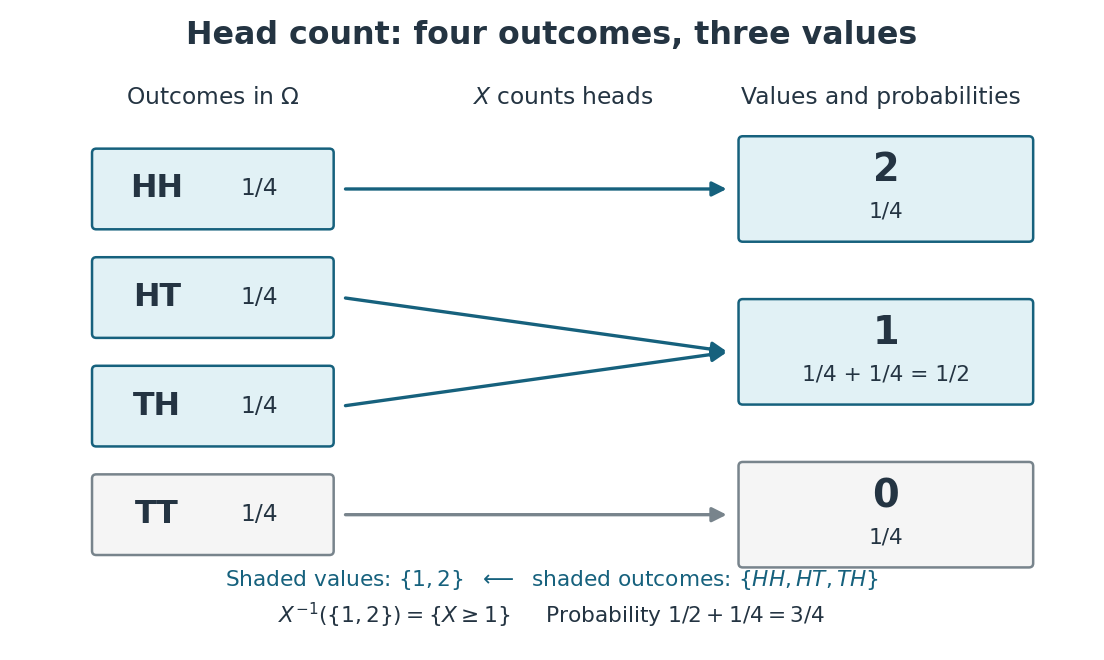
Head count merges outcomes into fibers and adds their probabilities
. The random variable sends to zero, both and to one, and to two. The inverse image of is the highlighted event of at least one head. Two arrows meeting at one explain its probability . Details.
Every event determined by is a union of complete fibers. There are such events, whereas the full power set of has . In particular, the first-head event is not determined by : it contains but excludes , although both give . Choosing an observable makes calculations simpler precisely by forgetting distinctions; the useful choice is one that retains the distinctions the question needs.
Two-sublattice Ising variational free energy 2026-10-14
Here . This free-energy density is the energy minus temperature times entropy of independent sublattice Ising spins. Since , stationarity yields the two-sublattice Ising mean-field approximation. Writing , the quadratic coefficients are for and for . The positive quartic coefficient in the staggered direction stabilizes the continuous transition. Unlike a log-cosh auxiliary potential, this variational expression can be minimized away from self-consistency.
On the stable zero-field branch , put . Differentiating the two-sublattice Ising mean-field approximation with respect to the uniform field gives and . Thus and . The true staggered magnetic susceptibility, , is a different response and diverges at the continuous transition. The factor is essential: the uniform response vanishes when the spins saturate at zero temperature.
In a two-generated two-step nilpotent group, use . Centrality of gives , so every word collects to . The multiplication of these collected expressions is . Relations on the central commutator can reduce modulo its order. To turn collection into a word problem for a group algorithm, one must also prove the independence of the remaining coordinates, for example by constructing a group with that cocycle multiplication.
In a steady inviscid planar incompressible flow, vorticity is constant along streamlines. A regular stream function supplies a local transverse coordinate, so locally depends only on . A global single-valued function needs the same value on every component of each level set. This can fail: gives the steady Euler shear with constant pressure, but while is respectively and .
For two distinct massless final particles, in the centre-of-mass frame. The invariant initial flux is . Their ratio gives the displayed differential cross-section. Equivalently the denominator is . Initial spins are averaged and final spins and colors summed when defining an inclusive unpolarized cross-section; averaging final colors would change the observable.
Clock hypothesis 2026-10-14
The clock hypothesis says that an ideal clock following a timelike curve measures its proper time: its instantaneous rate depends on velocity through , with no separate acceleration term. Acceleration still changes the world line and hence the accumulated proper time. A physical clock may suffer disturbances under forces or environmental changes, so experiments must distinguish its mechanism's errors from the geometric prediction.
Atomic clock 2026-10-14
Pontryagin-Thom collapse 2026-10-14
A compact smooth embedding has a tubular neighborhood identified with its normal bundle. Collapse the complement of its open disk neighborhood to the basepoint and identify the remaining quotient with the Thom space of that normal bundle. Pulling back its Thom class constructs a Gysin class. For a graph embedding into a product with Euclidean space, desuspending the auxiliary coordinates gives the corresponding wrong-way map.
Tubular neighborhood theorem 2026-10-14
A smooth embedded submanifold has a neighborhood diffeomorphic to a neighborhood of the zero section of its normal bundle, with the zero section identified with the submanifold. One may prescribe the normal-bundle splitting of the derivative along that section. Choose a Riemannian metric making the splitting orthogonal and use its normal exponential map: its derivative there is the required isomorphism, so the inverse function theorem supplies local diffeomorphisms. A sufficiently small, possibly varying, fibre radius makes these fit into a tubular neighborhood.
Tribes threshold window 2026-10-14
For tribes of size with and , the success probability under the p-biased product measure is . Its -quantile is . For fixed ,Thus the fixed-error window has order . For small fixed error the leading coefficient grows with , so the general Friedgut-Kalai sharp threshold theorem also has the correct error dependence up to absolute constants.
There are unlisted articles, also show them or only show them.