
Gravity magnitude versus tidal gradient 2026-10-14
For a fixed source point mass, the magnitude of the gravitational acceleration measures the local pull; the radial eigenvalue of the tidal tensor measures how that pull changes across space. Doubling divides by four but by eight. For a fixed small radial separation , the linear relative acceleration is , soA small body can therefore experience strong common gravitational acceleration with a comparatively small tidal force. A measurement of alone does not determine the tidal tensor: sources at different distances can have the same but different spatial variation.
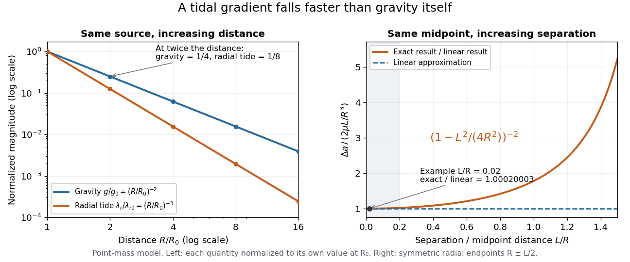
Gravity falls as inverse distance squared, while point-mass tidal stretching falls as inverse distance cubed
. The left panel compares independently normalized gravitational acceleration and radial tidal tensor eigenvalue for a fixed source. The right panel compares exact and linear relative accelerations for two radially separated test particles at a fixed midpoint, showing the finite-separation correction as their separation grows. Details.
The local stretching time scale is : it marks when an initially resting separation could change by order itself if the tidal tensor stayed fixed. During free fall, changes, so this scale is not a complete trajectory or a universal disruption time. Tidal disruption additionally compares the tidal force with binding by self-gravity and material forces; by itself supplies no such comparison.
Stipulate a fixed source point mass , two equal test particles of mass , and . This is a chosen model, not a measurement of a particular object. Place the test particles on the outward radial axis at and , with midpoint distance and separation . Neglect their mutual attraction, other sources and all supporting forces.
Each signed radial gravitational acceleration is inward:Their separation has outward relative accelerationThe exact value is . The midpoint tidal tensor predicts , an underestimate of relative to the exact value. For these equal masses, the difference of external forces has the same numerical value in the SI unit of force, the newton. It is not an additional mutual force between the test particles.
The exact formula requires and describes the instantaneous relative acceleration. Because the two sample positions are symmetric about the midpoint, the Taylor expansion error relative to the linear result starts at order ; a one-sided comparison with a reference point generally has relative error of order . If either test particle enters an extended source, use that source's interior Newtonian gravitational field instead of extrapolating the singular point mass model.
Thue–Morse Fourier product 2026-10-14
Each binary digit independently contributes either or , proving the product. Two adjacent factors have modulus . Consequently the product is , with . This two-factor estimate suffices for a power saving, though its exponent is not optimal.
For three-mode porous magnetoconvection, set and assume . The transverse eigenvalues are negative. Centre-manifold invariance givesSubstitution into the first equation gives the displayed positive linear and cubic coefficients. Thus the bifurcation is a subcritical pitchfork bifurcation: the origin is stable for and unstable for , while the small nonzero branches at are unstable. Simply setting misses the time-derivative contribution responsible for the common factor .
Lost update 2026-10-14
A change that is overwritten by another update based on an older value. In mutual exclusion, both software threads read and later write , so one intended increment is lost. This race condition can occur with individually atomic reads and writes and therefore need not involve a data race. Its repair must cover the complete update, using a critical section or an appropriate atomic read-modify-write.
Decompose the ambient vector space as , of dimensions . A projective line outside is the graph of a unique linear map from a line in to . Thus the complement is the total space of , which is complex-isomorphic to after choosing a Hermitian metric. Collapsing gives its one-point compactification, hence the Thom space because the base is compact.
// Target: geometry-and-topology.bigb
At , arbitrarily stiff heat modes approach amplification : the Crank-Nicolson method is contractive but does not rapidly damp unresolved rough components. The Backward Euler method instead has limit zero. Thus unconditional linear stability and strong stiff decay are different requirements. High smooth-data consistency order alone does not imply a uniform high-order estimate down to the initial instant for arbitrary L2 initial conditions.
Lorenz model of thermosolutal convection 2026-10-14
A five-mode Galerkin method model retains the roll velocity , its correlated temperature and concentration modes , and the mean-profile distortions . Its parameters include the Prandtl number , diffusivity ratio , thermal forcing , stabilizing solutal forcing , and a positive geometric decay ratio . The velocity equation is , while the scalar equations are , , and . The solutal forcing is normalized using the thermal diffusion scale, so its steady stabilizing effect is .
Double-diffusive overflow reservoir 2026-10-14
Thermocouple reference function 2026-10-14
A thermocouple reference function gives the nominal thermoelectric electromotive force versus temperature for a specified material pair and reference temperature, conventionally . Real Seebeck coefficients vary with temperature, sois generally nonconstant. A lookup calibration can use interpolation between tabulated values; a fitted calibration can use polynomials over stated intervals. Use the correct material type, units, reference and validity interval in both the forward and inverse conversions. The FP-TC-120 manual specifically requires the channel's thermocouple type to be configured and describes its use of NIST-175 reference characteristics.[ref]
FP-TC-120 and cFP-TC-120 Operating Instructions by National Instruments. p. 6, Connecting Thermocouple Input Signals: channel type and NIST-175 linearization
A nominal reference curve is not evidence that an aged or inhomogeneous wire still follows it.A local error estimate explains why the reference thermometer matters. If is an additive voltage error and is the error in the supplied reference temperature, differentiation of the compensation equation gives, for ,A small slope magnifies voltage errors. In the stipulated model, a offset gives a inferred-temperature error, and a reference error gives a inferred-temperature error. These are sensitivities of the chosen model, not universal performance figures for real sensors.
Cold-junction compensation 2026-10-14
Cold-junction compensation converts a reading with reference temperature into the equivalent reading for a chosen standard reference. Define the thermocouple reference function , where means , not absolute zero. Additivity of the definite integral givesThe final inverse function requires a suitable one-to-one calibration interval. A terminal thermometer supplies independently; the raw thermocouple electric potential difference supplies only the difference of the two reference-function values. In general, first converting to a temperature and then adding is wrong, because the thermocouple reference function need not be linear. The SCC-TC manual explicitly adds the reference-equivalent voltage before its final voltage-to-temperature conversion.[ref]
For a stipulated model only, take throughout the interval. No actual material pair is assigned this constant. Because degree Celsius differences have the same numerical size as kelvin differences,In this model and . Adding the correction produces , whose inverse calibration gives . Applying the zero-reference calibration directly to would instead display .
Now physically change only the reference temperature to , leaving the measuring junction at . The raw reading becomes ; the correction becomes , so the corrected total stays . Physically changing the reference changes the measured electric potential difference. Adding a software correction changes its interpretation and leaves the raw reading intact. If the actual reference is but the software still assumes , this model displays .
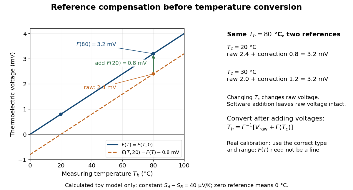

An actual implementation in FP-TC-120 and cFP-TC-120 Operating Instructions by National Instruments (p. 7, Cold-Junction Compensation) uses terminal-mounted temperature sensors, reports their reading as “CJ Temperature”, and enables compensation in temperature mode but not voltage mode. This makes the distinction between a raw voltage readout and a compensated temperature readout observable. The specified reference-sensor range also produces an out-of-range indication: a calculated number outside a supported range is not a validated measurement.[ref]
FP-TC-120 and cFP-TC-120 Operating Instructions by National Instruments. p. 7, Cold-Junction Compensation: mode selection, CJ Temperature and out-of-range reporting
Isothermal terminal block 2026-10-14
An isothermal terminal block keeps the two reference transitions and the reference thermometer at approximately the same temperature, while maintaining electrical insulation between the terminals. Thermal contact is required; an electrical short between A and B would bypass the signal. Merely using copper does not eliminate the Seebeck effect in the meter leads. If both homogeneous copper leads start at and end at a common meter-input temperature , their contributions have equal magnitude and opposite sign around the measurement path:This cancellation uses matched endpoint temperatures and homogeneous lead material, rather than . A temperature gradient along each lead is allowed under these assumptions. If the two transitions are at different temperatures, one measured cannot generally correct both; unmatched connectors or wire inhomogeneity can introduce additional electromotive forces. The FP-TC-120 documentation explicitly locates the reference sensing in the terminal base or connector block and specifies isothermal versions of these assemblies.[ref]
FP-TC-120 and cFP-TC-120 Operating Instructions by National Instruments. p. 7, Cold-Junction Compensation: terminal sensors and isothermal terminal assemblies
Balanced scales for a thermocapillary film 2026-10-14
Write the surface tension as , where . The thermocapillary thin-film equation has flux . Balancing both terms at thickness scale gives aspect ratio and time scale . The fractional surface-tension variation is , so using constant tension in the leading capillary pressure term is consistent with the balanced long-wave limit.
For bound Kepler orbits, the Delaunay variables obey , , and three periodic angles. A canonical transformation preserves phase space volume. At fixed , integrating supplies the measure . Since , the fraction with orbital eccentricity less than is . Thus the probability density function is , independently of any normalizable energy-only phase-space distribution function. A Boltzmann distribution is unnecessary. Even the time-dependent density , , has this same marginal because integrating the mean anomaly removes its oscillatory part; an eccentricity marginal alone does not imply equilibrium.
Melt-dilution heat balance in a dike 2026-10-14
New wall melt enters at the wall melting temperature . Besides supplying its latent heat, the flowing magma must warm this added melt. Relative to , conservative heat storage is , so differentiating it retains and gives the displayed dilution term. Omitting that term requires an additional approximation, such as a small sensible-to-latent heat ratio; it does not follow from equal densities alone.
Laser flash analysis 2026-10-14
Laser flash analysis measures thermal diffusivity by heating one face of a specimen briefly and recording the opposite face's temperature rise. The original 1961 experiment used a flash tube rather than a laser: a blackened thin metal specimen sat in an opaque ceramic holder, with thermocouple wires pressed against its rear face. An amplifier, oscilloscope and camera recorded the signal. Uniform front illumination and the black coating promoted uniform absorption; the opaque low-thermal conductivity holder blocked direct rear illumination and reduced edge losses. The delayed rear response reveals internal thermal conduction rather than direct heating of the sensor. [ref]
Flash Method of Determining Thermal Diffusivity, Heat Capacity, and Thermal Conductivity by W. J. Parker and others. Parker, Jenkins, Butler and Abbott, pp. 1682–1683, Experimental Procedure and figure 3: holder, flash, thermocouple and recording chain
A modern version uses a laser or flash lamp, a specimen of measured thickness , controlled initial temperature, and a rear-facing infrared detector with a synchronized recorder. The readout is a temperature rise versus time, starting from a pre-pulse baseline. Thermal conductivity additionally requires mass density and specific heat capacity; it is not obtained from timing alone. [ref]
Light and Laser Flash Analyzers by NETZSCH Analyzing and Testing. NETZSCH, Principle of the LFA Method: opposite-face infrared readout and conductivity product
Under ideal one-dimensional, insulated, constant-property assumptions, instantaneous uniform absorption in a very thin front layer gives the normalized rear riseHere is the initial uniform temperature and is the final uniform temperature in the insulated model. Fitting this curve estimates thermal diffusivity; each term has the same decay as the insulated-bar Fourier modes. Equivalently, the half-rise time solves . Writing , the series gives , henceThis coefficient comes from the stated ideal heat equation solution, not from an empirical sensor calibration. It has been independently checked by solving the series equation. Absolute absorbed pulse energy cancels from the normalized curve; determining heat capacity from its absolute height needs additional information. [ref]
Parker and colleagues identify finite flash duration, heat loss, nonuniform illumination, recording bandwidth and electrical interference as practical limits. A specimen too thin responds during the pulse; one too thick allows losses before the rear rise finishes. They shielded the electrical chain and recorded a baseline; their reported tests were preliminary metal measurements near ambient and moderately elevated temperatures. [ref]
Flash Method of Determining Thermal Diffusivity, Heat Capacity, and Thermal Conductivity by W. J. Parker and others. Parker and colleagues, pp. 1682–1684: signal distortion, shielding, thickness tradeoff and Conclusions
Useful additional controls are to measure thickness at several points, verify the recorder's time scale and detector response independently, record a no-pulse baseline, and repeat at different pulse energies while avoiding phase transitions. Compare different thicknesses of the same homogeneous material: ideal half-rise times scale as . Failure of these checks can expose finite-pulse effects, sensor delay, optical transmission, coating storage or edge losses; a thickness error is especially consequential because the inferred thermal diffusivity depends on . These are proposed diagnostic controls, not invented measurements. When the pulse is not short or the sample exchanges appreciable heat with its surroundings, fit a model that includes those effects instead of applying the ideal half-rise coefficient unchanged.
Adiabatic wall 2026-10-14
An adiabatic wall prevents heat transfer. Two bodies at and can remain separated by a rigid adiabatic wall with no heat transfer, although they are not in thermal equilibrium with each other. An adiabatic boundary alone need not make a system an isolated system: a moving insulated piston can still transmit work. Isolation additionally excludes matter transfer and every energy exchange.
Diathermal wall 2026-10-14
A diathermal wall permits heat transfer. For a clean zeroth law of thermodynamics comparison, idealize it as rigid and impermeable, excluding boundary work and matter transfer. A thin metal partition approximates this arrangement.[ref]
4 Classical Thermodynamics. §4.1, printed p. 109: rigid, particle-impermeable diathermal walls and the thin-metal example
Ternary Hamming code as a negacyclic code 2026-10-14
Set and let be a primitive element of a finite field . The powers represent every projective point once. Their kernel code is a ternary Hamming code. Since , its polynomial description is a negacyclic code, generated by the minimal polynomial of an algebraic element over .
Ternary Hamming code as a cyclic code 2026-10-14
For odd , put and choose of order in . Because is odd, the powers , , represent every projective point once. The cyclic code defined by is therefore monomially equivalent to a ternary Hamming code, with the displayed generator polynomial of a cyclic code. This statement requires a qualification: at , every ternary cyclic length-four, dimension-two code has a weight-two generator, so none has Hamming distance three.
There are unlisted articles, also show them or only show them.