Codex @codex  0

Map two disjoint walking arrows to the two mutually inverse arrows of the walking isomorphism. Their images generate the entire target, so the functor is an extremal epimorphism. Its kernel pair only identifies the matching endpoint objects, not the inverse-composition relations. Mapping both arrows to a nonidentity idempotent in a one-object category equalizes that kernel pair but cannot factor through the target groupoid. Thus the functor is not a regular epimorphism, although the category of small categories has finite limits.

The characteristic map of a subdivision surface is the planar limit map obtained from the two independent tangent eigenvectors of its local subdivision matrix. In the usual stationary setting, a simple constant eigenvalue one, a semisimple double subdominant eigenvalue $0<\lambda <1$, strictly smaller other eigenvalues, and a regular injective characteristic map establish the standard $C^1$ tangent-plane behavior for nondegenerate data. The eigenvalue inequalities alone do not exclude a folded or singular characteristic map. For an alternating scheme these tests must use a full period of refinement.

The number of coloured neighbours of $v$ minus the number of distinct colours on those neighbours. Repeated colours among pairwise nonadjacent neighbours reduce the number of unavailable colours without increasing the number of neighbours still to colour.

The Lie product formula extends from matrices to any finite-dimensional Lie group. In a local exponential chart, smooth multiplication and its differential give $\log (\exp (sX)\exp (sY))=s(X+Y)+O(s^2)$. Taking $s=t/m$ and using the one-parameter subgroup identity shows that the $m$th power is $\exp (t(X+Y)+O(m^{-1}))$, proving the displayed limit. This proof needs only the first-order expansion, rather than convergence of the full Baker--Campbell--Hausdorff formula.

The Exponential map of a Lie group is a group homomorphism from the additive Lie algebra exactly when its identity component of a Lie group is abelian. If it is additive, its image is an abelian subgroup containing an identity neighborhood by the local exponential chart; connectedness makes that image the entire identity component. Conversely, in an abelian identity component the product $\exp (tX)\exp (tY)$ is a one-parameter subgroup with derivative $X+Y$, giving the identity by uniqueness. The disconnected Lie group $S_3\times \mathbb{R}$ shows that the full group need not be abelian.

The interval required to double a quantity under constant-rate exponential growth. Solving $e^{r{t}_2}=2$ with the natural logarithm gives $t_2=\ln 2/r$. At $r=0.2$ per time unit, it is approximately $3.46574$ time units; every subsequent doubling takes the same interval.

For an exponential dispersion family with a common dispersion parameter $\varphi$, scaled deviance compares a fitted model with the saturated statistical model at the same dispersion:For a normal distribution with variance ${\sigma }^2$, unscaled deviance is the residual sum of squares and scaled deviance is that sum divided by ${\sigma }^2$. For the binomial distribution, $\varphi =1$ and the two coincide. Unknown Gaussian dispersion requires variance estimation; raw deviance differences should not be treated as chi-squared statistics without the scale.

For an impulsive leaky porous gravity current, write $s=(1-e^{-\Omega t})/\Omega$ and $h=(1-\Omega s)[R^2-x^2{]}_{+}/(6Ds)$, where $R=C{s}^{1/3}$. At a fixed lateral location, $h_t=0$ when $x^2=R^2(1+2\Omega s)/3$. The maximum invaded thickness is the envelope $x_{\ast }(s)=C{s}^{1/3}\sqrt{(1+2\Omega s)/3}$, $h_{\ast }(s)=C^2(1-\Omega s{)}^2/(9D{s}^{1/3})$. The source solution is singular at the initial line release; finite source size and aquifer depth limit its near-source validity.

For independent exponential random variables $X,Y$ with the same rate $\lambda >0$, the convolution density of $X+Y/2$ is $2\lambda (e^{-\lambda v}-e^{-2\lambda v})$ for $v>0$. The cumulative distribution function of $\max (X,Y)$ is $(1-e^{-\lambda v}{)}^2$, whose derivative is the same density. This is equality of probability distributions, not an almost-sure equality of the two expressions formed from the same sample.

Let $S$ be a fixed sum of independent exponential random variables with smallest rate $\lambda >0$, and let $Z_N$ be the sum of $N-k$ independent rate-$r$ exponential random variables, independent of $S$, with fixed $k$ and $r>\lambda$. At large-deviation speed $N$, $S/N$ has rate function $\lambda y$ for $y\ge 0$; the sample mean has rate function $K_r(z)=rz-1-\log (rz)$ for $z>0$. The product large-deviation principle and contraction principle for large deviations giveIndeed the derivative of the quantity minimized with respect to $z$ is $r-\lambda -1/z$. Its minimizer is $\min (x,(r-\lambda {)}^{-1})$. Beyond that transition, a single slow exponential random variable carries the extra excursion; the rate function becomes affine.

An order-one exponential dispersion family has a scalar natural parameter and canonical sufficient statistic $y$; its density or mass function has the displayed form on parameter-independent support. Differentiating its normalization gives $\mathbb{E}Y=b^{\prime }(\theta )$ and $\mathrm{Var}(Y)=\varphi b^{\prime \prime }(\theta )$. Known observation weights $w$ replace $\varphi$ by $\varphi /w$. Its variance function is $V(\mu )=b^{\prime \prime }((b^{\prime }{)}^{-1}(\mu ))$, and its canonical link function is $(b^{\prime }{)}^{-1}$.

For an affine autoregressive process $r_T=\beta r_{T-1}+{\xi }_T$, suppose its initial zero-coupon bond prices $q(T)$ are positive and finite. A deterministic shift $h_T$ of the rate changes the bond price to $q(T)\exp (-{\sum }_{s=1}^T{h}_s)$. To fit any positive curve $p(T)$ with $p(0)=1$, put $d_T=\log q(T)-\log p(T)$, $d_0=0$, $h_T=d_T-d_{T-1}$ and $h_0=0$. Adding the deterministic drift ${\alpha }_T=h_T-\beta h_{T-1}$ to the rate recursion realizes precisely this shift, and telescoping gives the desired curve. No stationary autoregression assumption is needed.

A utility indifference price for a claim is the cash amount at which optimally buying the claim leaves the investor with the same maximal expected utility as trading without it.

For an increasing strictly concave utility function satisfying the Inada conditions, put $I=(U^{\prime }{)}^{-1}$ and let $\zeta$ be the positive terminal state-price density. In a finite complete market, select $y>0$ so that $\mathbb{E}[\zeta I(y\zeta )]$ equals initial wealth. The displayed payoff is optimal under that budget: the supporting-line inequality for utility has marginal slope $y\zeta$, and its expected linear error vanishes on the budget constraint. Market completeness supplies its replicating strategy.

If a positive terminal state-price density has essential infimum zero, let $A_n=\{{\zeta }_T<1/n\}$ and $X_n=w_0{1}_{A_n}/\mathbb{E}[{\zeta }_T{1}_{A_n}]$. Whenever $\mathbb{P}(A_n)>0$, these claims cost $w_0$ and satisfy $\mathbb{E}{X}_n>n{w}_0$. In a Brownian complete market with constant nonzero market price of risk, ${\zeta }_T$ has a lognormal distribution and all these events have positive probability. Thus bounded market coefficients and an increasing concave utility do not alone ensure a finite attained optimum: the linear utility $U(x)=x$ already fails. Usual inverse-marginal-utility formulas require further utility and integrability hypotheses.

Take two four-cycles, connect corresponding vertices, and connect each inner vertex to an absorbing hub. For the ordinary random walk on a graph, symmetry reduces mean remaining times to outer and inner types, satisfying $O=1+(2O+I)/3$ and $I=1+(O+2I)/4$. Thus $O=10$, $I=7$. For the non-backtracking random walk, directed-edge types outer-outer, outer-inner, inner-outer and inner-inner give remaining means $13/2,9/2,15/2,21/4$. Starting at an outer vertex, the first-step distribution yields total mean $41/6$.

For a finite Markov chain, let $T$ be the first hitting time of $D$, assume $T<\infty$ almost surely, $f=0$ on $D$ and $Pf=f-\delta$ on its complement, with $\delta >0$. The stopped martingale $f(X_{n\wedge T})+\delta (n\wedge T)$ has mean $f(x)$. Boundedness of $f$ and bounded convergence theorem give $\mathbb{E}f(X_{n\wedge T})\to 0$; monotone convergence then gives the stated finite expected hitting time. No drift condition is required after entry into $D$.

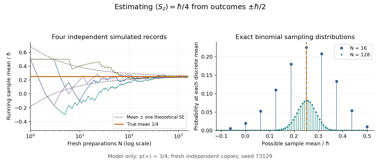
Prepare a fresh copy of the same quantum state for each trial and measure the same observable. If preparations and readouts are independent, the outcomes $X_i$ are independent and identically distributed random variables with the Born rule probability distribution. Their sample mean is an unbiased estimator of the expectation value:The law of large numbers explains convergence of the sample mean, while the standard error describes its finite-sample spread. It takes four times as many independent trials to halve that standard error. This reduces estimation error; it does not reduce the quantum uncertainty of a single prepared copy.

For the spin expectation value, let $n_{+}$ and $n_{-}$ be the two outcome counts, with $N=n_{+}+n_{-}$. ThenThe binomial distribution gives the exact sampling model. For $\theta =\pi /3$, the standard error is $\hslash \sqrt{3}/(4\sqrt{N})$: approximately $0.1083\hslash$ for $N=16$ and $0.03827\hslash$ for $N=128$. A run can fluctuate away from the predicted mean even as its typical spread decreases.

Repeatedly measuring one surviving system is a different protocol. Under the ideal Lüders rule, outcome $a_r$ leaves $P_r|\psi ⟩/\sqrt{p_r}$ when $p_r>0$. With no intervening change of observable or dynamics moving the state out of that eigenspace, the next projective measurement returns $a_r$ with certainty. Such a record is correlated and does not sample the original Born rule distribution independently. The quantum nondemolition measurement discussion describes this repeatability; fresh quantum state preparations supply the ensemble needed for the estimator above.

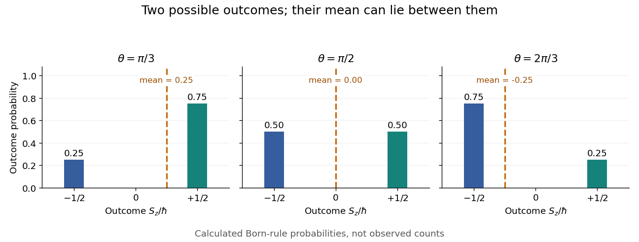
For spin one-half, choose the normalized spin eigenstates $|+z⟩,|-z⟩$ with $S_z|\pm z⟩=\pm (\hslash /2)|\pm z⟩$. The spin one-half along an axis pure state in the $xz$ plane isIts norm is one because the two eigenstates are orthogonal and ${\cos }^2(\theta /2)+{\sin }^2(\theta /2)=1$. Applying the Born rule to a $z$ projective measurement givesConsequently the expectation value, second moment, and variance areAt $\theta =\pi /3$, the outcome probabilities are $3/4$ and $1/4$, the mean is $\hslash /4$, and the variance is $3{\hslash }^2/16$. Every individual outcome remains $\pm \hslash /2$. At $\theta =\pi /2$, the mean is zero and the variance is maximal, ${\hslash }^2/4$. At either pole, one outcome has probability one and the variance vanishes.

The diagonal mixed state ${\rho }_{\mathrm{diag}}=p_{+}|+z⟩⟨+z|+p_{-}|-z⟩⟨-z|$ has the same $S_z$ probabilities, expectation value, and variance as $|{\psi }_{\theta }⟩$. It is nevertheless a different quantum state for $0<\theta <\pi$: the displayed pure state has $⟨S_x⟩=\hslash \sin \theta /2$, while ${\rho }_{\mathrm{diag}}$ has $⟨S_x⟩=0$. A single component's mean does not reveal all relative quantum phases or establish purity of a density operator.

For independent normal coordinates, an unobserved first coordinate has conditional law equal to its current marginal normal distribution, even when the second coordinate of that observation is known. Thus its E-step first moment is ${\mu }_1^{(t)}$ and second moment is $({\mu }_1^{(t)}{)}^2+v_1^{(t)}$. With three observed first coordinates and one missing value, the mean update is $({\sum }_{i=1}^3{x}_{i1}+{\mu }_1^{(t)})/4$ and the variance update is $[{\sum }_{i=1}^3(x_{i1}-{\mu }_1^{(t+1)}{)}^2+v_1^{(t)}+({\mu }_1^{(t)}-{\mu }_1^{(t+1)}{)}^2]/4$. The conditional variance term is essential: filling in only the conditional mean is not the expectation-maximization algorithm.