
Measured output 2026-10-14
The measured output is the information about the plant output available to the controller. It may differ from the actual plant output because of measurement noise or feedback delay. In the ideal examples , so the controller observes the actual current state exactly.
Curved spacetime gamma matrices 2026-10-14
An orthonormal coframe converts fixed flat gamma matrices to coordinate-index Clifford multiplication. Its metric identity gives the curved anticommutation relation. The spin connection is chosen so that these matrices are covariantly constant under the combined spin and tensor connection, which is the tetrad postulate in Clifford form.
Zernike polynomials 2026-10-14
The real Zernike polynomials form an orthogonal polynomial basis on the unit Euclidean disk, with radial factor and angular factor or . Here and is even. They decompose wavefront errors into modes useful for optical correction. Normalizations differ, so coefficients should specify the chosen convention.
Orthogonality forces many interior zeros 2026-10-14
If a nonzero continuous real function on an interval is orthogonal to every polynomial of degree below , it has at least distinct interior zeros. If it had only finitely many zeros and fewer than sign changes, multiply it by the product of linear factors at its sign-changing zeros. The product has constant sign and is nonzero on an open interval, so its integral cannot vanish. Orthogonality to this degree-below- polynomial contradicts that conclusion. Infinitely many interior zeros already satisfy the assertion. Orthogonal polynomials of respective degrees form a basis of the needed polynomial space.
Kravchuk polynomials Created 2026-10-14 Updated 2026-10-18
These polynomials are orthogonal for a binomial distribution weight and encode the coefficient transformation in the MacWilliams identity. Their generating function follows by expanding the two factors:For binary linear codes, . Expanding the factors gives , where binomial coefficients outside their usual integer range are zero. Orthogonality follows by multiplying generating functions and summing over with weight : the result is , whose coefficient of is zero for and for .
Determinant-twist projection in odd dimension Created 2026-10-14 Updated 2026-11-05
For real orthogonal matrices in odd dimension , multiplying by their determinant defines a group homomorphism from onto . Scalar factors commute, so , while . The map fixes and has kernel . Since is central and has determinant in odd dimension, . In even dimension the same expression does not map every orthogonal matrix into the special orthogonal group.
Cartan–Dieudonné theorem 2026-10-14
Every orthogonal transformation of a finite-dimensional nondegenerate quadratic space over a field of characteristic different from two is a product of at most its dimension many hyperplane reflections. In the real positive-definite case, a reflection normal to sends to whenever . Composing with that reflection fixes and leaves an orthogonal transformation of , so induction proves the bound. Each reflection has determinant minus one, hence orientation-preserving transformations use an even number of reflections.
Orthogonal group as a regular level set Created 2026-10-14 Updated 2026-11-05
The smooth Gram map takes real matrices to symmetric matrices. At an orthogonal , its derivative sends to any prescribed symmetric matrix . The regular level set is therefore a smooth manifold of the displayed dimension.
// Target: geometry-and-topology.bigb
Localization condition for the fastest orthogonal-field interface mode Created 2026-10-14 Updated 2026-11-05
For the density jump of a magnetic pressure discontinuity in an isothermal atmosphere, with , the fastest Rayleigh-Taylor instability has and . Its vertical decay length is . Hence localization relative to both common scale heights requires . This also makes its growth speed small compared with the isothermal sound speed. If , the ideal sharp-interface dispersion relation instead has unbounded growth as : there is no finite maximizing mode.
Squire's theorem 2026-10-14
For temporal normal-mode stability of a viscous parallel shear flow, any unstable three-dimensional mode maps by the Squire transformation to an unstable two-dimensional mode at a no larger Reynolds number. Hence the first temporal modal instability occurs among two-dimensional disturbances. The theorem does not exclude three-dimensional transient growth or forced responses.
Potential of a uniform spherical source 2026-10-14
For a uniform spherical source of radius , the origin-regular radial Poisson equation gives inside and outside. Integrating radially, imposing at infinity and continuity at , givesThe potential and its normal derivative are continuous at the interface, so its distributional Laplacian has no surface delta contribution. The classical equation holds off the interface and the source equation holds almost everywhere and distributionally.
Arborescence (graph theory) Created 2026-10-14 Updated 2026-11-05
An arborescence is a rooted tree with each edge oriented away from its root. There is a unique directed path from the root to every vertex; equivalently the root has indegree zero and every other vertex has indegree one. Reversing all edges gives an in-arborescence, with unique directed paths toward the root.
For , every -vertex arborescence embeds in every tournament on vertices. The half-sparse median-order embedding proves this by repeatedly extending an outward leaf. Reversing the tournament and the arborescence gives the corresponding in-arborescence statement. The restriction matters: a one-vertex arborescence needs a nonempty host, while would give an empty host.
For a source-rooted oriented tree, let count edges pointing towards the root and let count nonempty connected components formed by those edges. A half-sparse median-order embedding exists in vertices. Remove forward leaves, or remove a terminal backward component of order and replace it temporarily by outward leaves. Their images contain an in-arborescence copy of the component. Choose the direction and root to minimize lexicographically; this makes the root a source and gives unless the tree is already an arborescence. The stated bound follows.
Ore theorem Created 2026-10-14 Updated 2026-11-05
A multiplicative set of regular elements of a ring admits a right ring of fractions exactly when it satisfies the right Ore condition. The resulting localization embeds the original ring, inverts , and expresses every element as . For denominators that can be zero divisors, an additional denominator reversibility condition is required.
Periodic solution Created 2026-10-14 Updated 2026-10-14
A periodic solution is a solution of a differential equation which is a periodic function: for some , at every time. This demands repetition of the state, rather than merely repetition of the coefficients in the differential equation. A nonconstant periodic solution of an autonomous differential equation traces a periodic orbit; constant equilibrium points are also periodic functions, so they must be excluded when asserting absence of periodic orbits.
For an explicit example, consider the initial value problemIts coefficient has period . Taking a logarithmic derivative and then applying integration givesDirect differentiation verifies both the differential equation and the initial condition. After one coefficient period,Thus the repeating coefficient generally produces a repeating shape with a changed amplitude. With , the three cases have one-period factors approximately , respectively. Only gives a periodic solution with this initial condition. For the positive solution of a differential equation tends to zero, and for it tends to infinity; neither can have any positive period. The zero solution of a differential equation, obtained with a different initial condition, is periodic for every .
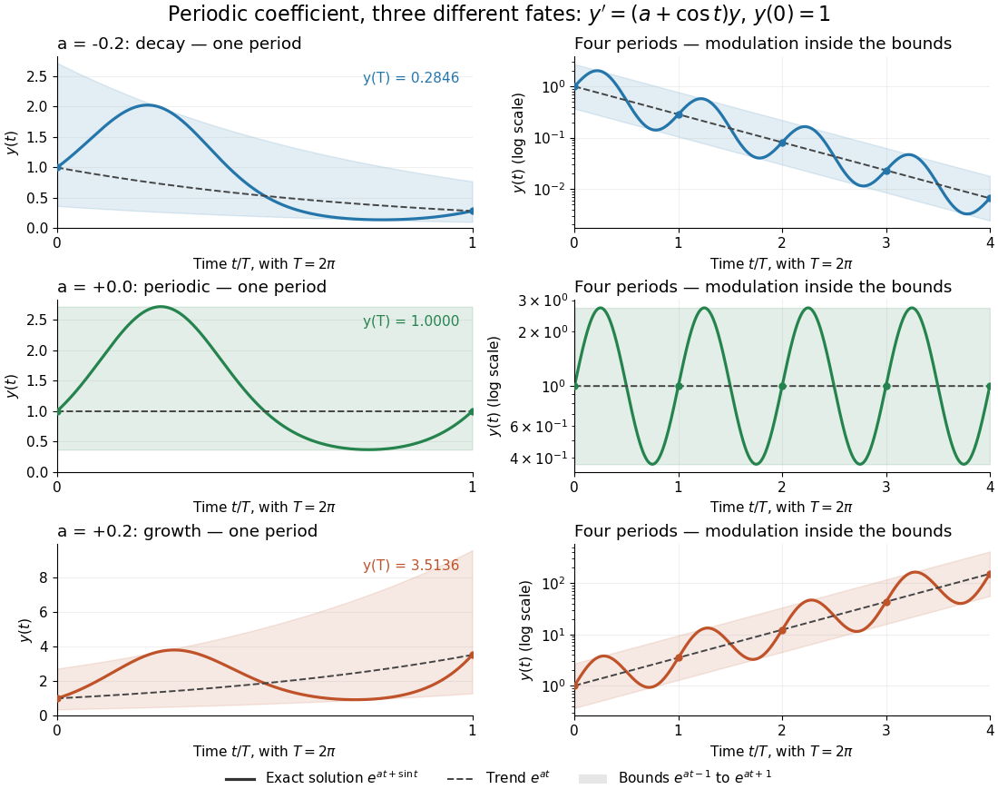
One repeating coefficient can produce decay, periodic motion, or growth
. The original example , , shown over one coefficient period and four coefficient periods. Shading marks the bounds , and dashed curves mark . The right column uses a logarithmic vertical scale. Details.
The exponential function separates two roles:For , even the decaying case initially rises, because . The growing case has intervals of decline, because becomes negative. This is the distinction between the instantaneous logarithmic derivative and the Floquet growth rate measured over many periods.
More generally, for a real continuous periodic function of period , the scalar linear differential equation hasA nonzero solution of a differential equation is -periodic exactly when , or equivalently when the coefficient has zero integral over a period. This scalar calculation is the simplest example of a Floquet multiplier.[ref]
Complex ordinary differential equation 2026-10-14
A first-order ordinary differential equation with complex independent and dependent variables is solved by a holomorphic function on an ordinary domain, and its analytic continuation can have branch points. A holomorphic right-hand side gives local existence and uniqueness by the integral contraction mapping used in the Picard-Lindelöf theorem.
Painlevé equation Created 2026-10-14 Updated 2026-11-05
The six Painlevé equations are distinguished nonlinear second-order ordinary differential equations whose solutions have no movable branch points: singularities whose positions depend on the initial data can be poles, but not branching singularities. Their solutions are called Painlevé transcendents. The first equation is , while the Painlevé II equation is . The six families include parameters and admit special solutions at particular parameter values; they are not merely six individual functions.[ref]
NIST Digital Library of Mathematical Functions. §32.2(i), equations 32.2.1–32.2.6 and the Painlevé property discussion
Second-order differential equation 2026-10-14
A second-order ordinary differential equation involves a second derivative as its highest derivative. In explicit form , introducing converts it into the first-order system , . Under local regularity and Lipschitz continuity in the dependent variables, an initial value problem is specified by both and . The linear case is a second-order linear differential equation.
First integral of an ordinary differential equation Created 2026-10-14 Updated 2026-10-18
A first integral of is a differentiable function whose value is constant along solutions through every time and state in its domain. The chain rule makes this equivalent to the displayed pointwise identity. For with symmetric , it becomes . This identity at the implicit stage is what proves exact Runge-Kutta conservation of quadratic invariants for the implicit midpoint rule. Invariance asserted only on the image of one initial-time flow needs that image to contain the stage under consideration.
Ordinal arithmetic 2026-10-14
Ordinal arithmetic defines addition, multiplication and exponentiation of ordinals through order types or transfinite recursion. The usual operations need not be commutative. Natural sum and natural product instead combine Cantor normal forms and are commutative; the Hessenberg natural sum is the natural addition operation.
There are unlisted articles, also show them or only show them.