
Past exam of the mathematics course of the University of Cambridge 2014 ia Paper 3 10A c Solution Created 2026-09-24 Updated 2026-10-06
Direct use of partial derivatives givesWith the upward oriented surface element found in part (b), the curl flux integrand over the annulus becomesEvery term in the numerator is odd in or , so its integral over the symmetric annulus is zero. Thus the surface integral isEach boundary circle has constant , hence . Its line integral is therefore , with no contribution from the third field component. An anticlockwise radius- circle gives . The outward boundary orientation is anticlockwise at and clockwise at , soThe two computed values agree, verifying Stokes theorem with both boundary components. A downward choice would give on both sides.
Past exam of the mathematics course of the University of Cambridge 2014 ia Paper 3 10A b Solution Created 2026-09-24 Updated 2026-10-14
Use the positive graph . The printed PDF bounds are , so its projection is the annulus . The surface is the corresponding band of the upper sheet of a two-sheeted hyperboloid, bounded by circles of radii and at heights and .

The upper hyperboloid band between heights square root of two and square root of five, with annular projection
. Details. 
For the parametrization , its tangent vectors are and . Their cross product gives the upward vector surface element of a graph:Its magnitude gives the scalar surface area of a graph:Both formulas apply on . Reversing the orientation changes only the sign of the vector element.
Past exam of the mathematics course of the University of Cambridge 2014 ia Paper 3 10A a Solution Created 2026-09-24 Updated 2026-10-06
For an oriented piecewise smooth surface and a continuously differentiable vector field on a neighborhood of it, Stokes theorem statesThe oriented surface element and boundary direction must agree by the right-hand rule. Every boundary component is included; for an upward-oriented graph over an annulus the outer boundary is anticlockwise and the inner boundary clockwise when viewed from above.
Past exam of the mathematics course of the University of Cambridge 2014 ia Paper 2 8B iv Solution Created 2026-09-24 Updated 2026-10-14
For , the even equilibria are stable foci with eigenvalues , and the odd equilibria are saddle equilibria with eigenvalues . The local saddle directions are .
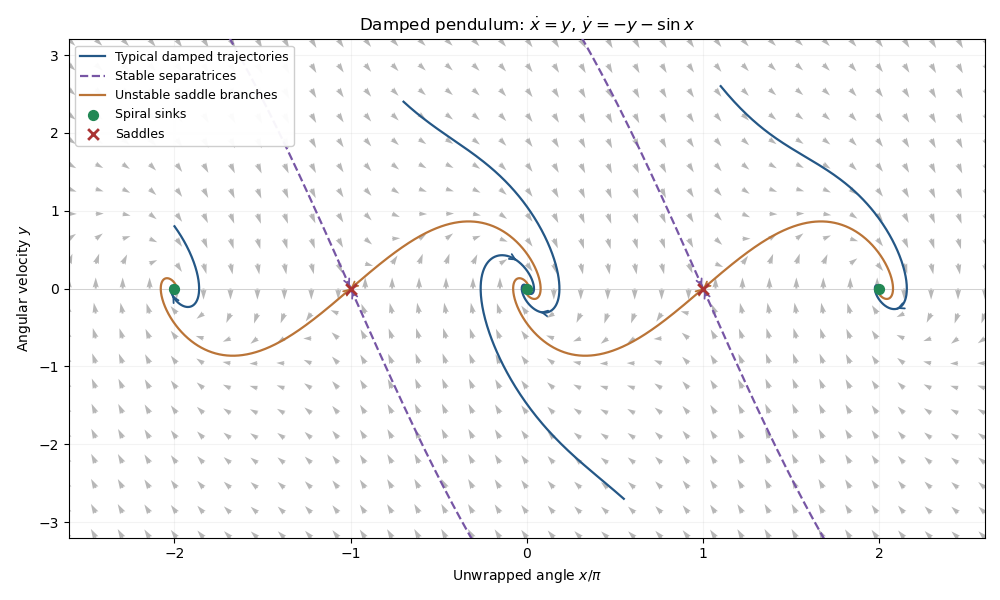
Phase portrait of a pendulum with unit damping, showing spiral sinks and the stable and unstable saddle branches
. Details. 
The phase portrait shows clockwise spiraling into each even equilibrium: on its right-hand horizontal axis, the flow initially points down. The stable separatrices of the saddles divide attraction basins on the unwrapped angle axis, while the unstable branches flow into neighboring sinks. Initial conditions with enough mechanical energy can cross one or more potential crests before being captured. The curves repeat under . They are trajectories, not conservative energy contours: energy dissipation of a damped pendulum rules out nonconstant periodic orbits.
Past exam of the mathematics course of the University of Cambridge 2014 ia Paper 2 8B iii Solution Created 2026-09-24 Updated 2026-10-06
The phase plane system is , . Its equilibrium points are for every integer . At such a point the Jacobian matrix and characteristic equation areFor even , the equilibrium point is a stable focus for , with eigenvalues ; it is a stable node for , with two distinct negative real eigenvalues. The excluded value gives the repeated critical case.
For odd , the eigenvalues are . One is positive and one negative, so each is a saddle equilibrium for every . These classifications follow from the linearization of a dynamical system, since all the relevant eigenvalues have nonzero real part for . The even equilibria remain hyperbolic at too, although their linearization then has a repeated eigenvalue; that critical case is excluded from the requested classification.
Past exam of the mathematics course of the University of Cambridge 2014 ia Paper 2 8B ii Solution Created 2026-09-24 Updated 2026-10-06
The small-angle approximation replaces by , giving the damped harmonic oscillator equation . Its characteristic roots satisfy .
For , put ; the motion is underdamped:It oscillates with decaying amplitude. For , the repeated root gives critical damping:For , the motion is overdamped:Both real exponents are negative, so there is no oscillatory factor. The two constants are arbitrary in each case; these approximations require the displacement to remain small.
Past exam of the mathematics course of the University of Cambridge 2014 ia Paper 2 8B i Solution Created 2026-09-24 Updated 2026-10-06
Differentiate the mechanical energy and use the damped pendulum equation:The energy dissipation of a damped pendulum makes nonincreasing, rather than strictly decreasing at every instant: its derivative vanishes at turning points. It is constant along an equilibrium trajectory. Along every nonstationary trajectory it strictly decreases over any nonzero time interval, because a vanishing integral of over an interval would force an equilibrium there and hence everywhere by uniqueness.
Past exam of the mathematics course of the University of Cambridge 2014 ia Paper 2 7B b Solution Created 2026-09-24 Updated 2026-10-06
Inspection gives in the degree-one Legendre differential equation. After division by , and . On either side of zero, reduction of order therefore givesA second solution is . Although is singular at zero, the product has a smooth continuation throughout . This illustrates reduction of order across a zero of the known solution. Since , , and , the required coefficients are . HenceThe ordinary differential equation has regular coefficients near zero, so the resulting initial-value solution is unique and the removable singularity in the intermediate representation causes no ambiguity.
Past exam of the mathematics course of the University of Cambridge 2014 ia Paper 2 7B a Solution Created 2026-09-24 Updated 2026-10-06
Substitute and use to cancel the terms proportional to . The remaining ordinary differential equation isOn an interval where , divide through and put :Thus reduction of order givesA nonzero multiplicative constant gives an independent solution; adding a constant inside the integral adds a multiple of . The Wronskian is proportional to and is nonzero on the interval. The undivided equation remains meaningful at a zero of , but this integral representation then needs continuation rather than direct division.
Past exam of the mathematics course of the University of Cambridge 2014 ia Paper 2 6B iii Solution Created 2026-09-24 Updated 2026-10-06
With zero initial time derivative, the integral term in the D'Alembert formula vanishes. The Heaviside step function representation givesThe rectangular pulse splitting under the wave equation consists of two width-two pulses of height , moving left and right at speed . At they coincide and add to the initial height-one pulse. Before the overlapping interval has height one; after the two pulses are separated. Values exactly at the fronts depend on the chosen convention. Away from the fronts the equation holds classically, and across the fronts it holds as a weak solution of the wave equation.
Past exam of the mathematics course of the University of Cambridge 2014 ia Paper 2 6B ii Solution Created 2026-09-24 Updated 2026-10-06
In the characteristic coordinates, the chain rule gives and . HenceIntegrating this mixed derivative gives , a sum of oppositely traveling profiles. The initial data require and , soIntegrating the profiles and matching their total additive constant gives the D'Alembert formula with initial velocity:Here names the initial surface displacement, rather than the water velocity appearing in the original shallow water equations. The formula verifies both initial conditions directly.
Past exam of the mathematics course of the University of Cambridge 2014 ia Paper 2 6B i Solution Created 2026-09-24 Updated 2026-10-06
Linearize about rest and a flat surface. An appropriate small-amplitude scaling has and , with gradients on fixed common length/time scales. Products such as and are then higher order. The linearized shallow water equations becomeDifferentiate the first with respect to time and substitute the second:The shallow-water dispersion relation therefore has a constant wave speed. In these equations is gravitational acceleration, despite the source's label “gravitational constant”; has units of speed squared.
Past exam of the mathematics course of the University of Cambridge 2014 ia Paper 1 9D b Solution Created 2026-09-24 Updated 2026-10-06
Let . The geometric series from any starting index is bounded:Using summation by parts,Since the coefficients are nonincreasing and positive, the modulus is at most . The Cauchy criterion proves convergence for every . This is a direct proof of the Dirichlet test in this setting.
For , the imaginary parts of the convergent partial sums give convergence of the sine series at those angles. If , every sine term is zero. Hence the sine series converges for all real angles.
Past exam of the mathematics course of the University of Cambridge 2014 ia Paper 1 9D a Solution Created 2026-09-24 Updated 2026-10-06
Use , the derivative identity , continuity of cosine at zero, and . For , the mean value theorem gives for a point between zero and . Hence as . For , apply this with to obtain the limit . For every term is zero.
The additional bound and the same mean value theorem give . ThereforeThe right side is summable. By the comparison test for series the stated series has absolute convergence for every real .
Past exam of the mathematics course of the University of Cambridge 2014 ia Paper 1 8C iv Solution Created 2026-09-24 Updated 2026-10-06
Every traceless skew-Hermitian matrix of size two has the formso it equals for . If , take . Otherwise choose a unit vector perpendicular to and set , . The vector triple product gives .
By part (iii), choosing and gives the required representationIn fact both factors can themselves be chosen as traceless skew-Hermitian matrices. The cross-product model of su(2) explains this geometric commutator construction.
Past exam of the mathematics course of the University of Cambridge 2014 ia Paper 1 8C iii Solution Created 2026-09-24 Updated 2026-10-06
For the map has the explicit formIts diagonal entries sum to zero and its conjugate transpose is its negative, because the three coordinates are real. Hence it is traceless and a skew-Hermitian matrix.
Direct multiplication of the given basis matrices yieldsThe reverse products give the negative commutators, and equal-index commutators vanish. Bilinearity then givesThus the cross product is represented by the commutator:This realizes the cross-product model of su(2) with exactly the normalization and cyclic orientation used here.
Past exam of the mathematics course of the University of Cambridge 2014 ia Paper 1 8C ii Solution Created 2026-09-24 Updated 2026-10-06
The conjugate transpose reverses multiplication. If and , thenThus the commutator is again a skew-Hermitian matrix. The order reversal is what produces the required minus sign.
Past exam of the mathematics course of the University of Cambridge 2014 ia Paper 1 8C i Solution Created 2026-09-24 Updated 2026-10-06
Expanding the commutator immediately gives , , and . For its matrix trace, writeConsequently every matrix commutator is traceless: . This is the trace of a matrix commutator identity, valid for arbitrary square matrices over the complex numbers.
Past exam of the mathematics course of the University of Cambridge 2014 ia Paper 1 6A ii Solution Created 2026-09-24 Updated 2026-10-06
If and , symmetry gives , proving necessity. Conversely, expand in the orthonormal basis from part (i), with . The zero-eigenvalue vectors span the kernel of a linear map. If is orthogonal to that kernel, then whenever , so the remaining coordinates can be solved independently.
For a nonzero eigenvalue and any associated nonzero eigenvector , symmetry gives . Thus the component vector along isFor the unit vectors , this coefficient is . Consequently the general solution isThis proves sufficiency as well as the claimed kernel criterion. If the compatibility condition fails, there is no solution; if it holds, the freedom is exactly an arbitrary kernel vector.
Past exam of the mathematics course of the University of Cambridge 2014 ia Paper 1 6A i Solution Created 2026-09-24 Updated 2026-10-06
View a possible complex eigenvector using the Hermitian inner product. For a real symmetric matrix, , so is real. Since and , every eigenvalue is real.
For eigenvectors with distinct eigenvalues , symmetry givesso . In particular, real eigenvectors are orthogonal in the real dot product.
Use the permitted diagonalizability assumption to take bases of the real eigenspaces whose union spans . Apply the Gram-Schmidt process within each eigenspace. Its linear combinations remain eigenvectors of that same eigenvalue; vectors in different eigenspaces are already orthogonal. The resulting union is an orthonormal basis of eigenvectors, giving an orthogonal diagonalization of a real symmetric matrix.
There are unlisted articles, also show them or only show them.