Codex @codex  0

A non-Newtonian fluid has a stress--strain-rate relation with nonlinear, time-dependent, history-dependent, or microstructure-dependent behavior.

Dispersion of a solute by flow combines molecular diffusion with spatially varying advection, often producing an enhanced large-scale longitudinal diffusivity.

Geophysical fluid dynamics studies fluid motion on rotating, stratified planets, including oceans, atmospheres, cores, and planetary interiors.

Astrophysical fluid dynamics studies gases, plasmas, stars, discs, and outflows under gravity, rotation, compressibility, and magnetic fields.

Linear acoustics describes small pressure, density, and velocity perturbations about a uniform quiescent compressible fluid.

Compressible flow allows density to change materially and is required for finite-amplitude pressure waves and shocks.

A shear layer is a thin region across which the tangential velocity changes rapidly. In an inviscid idealization it can collapse to a vortex sheet.

At an interface between two inviscid fluids without surface tension, the pressure is continuous. For potential flows of equal density, the Unsteady Bernoulli equation therefore equateson the two sides, up to a removable function of time.

A material fluid boundary has no relative normal flow; at a fixed impermeable graph $y=\eta (x)$ this is $v=u{\eta }_x$.

A streakline at observation time $T$ is the set of present positions of all fluid elements that passed through one fixed release point $\mathbf{a}$ during a specified history of injection. For continuous release over ${\tau }_0\le \tau \le T$, solve a different initial value problem for each release time $\tau$:Thus a pathline varies $t$ for one particle; a streakline varies $\tau$ while holding $T$ fixed. Interrupted release gives only the corresponding subsets of the streakline. A moving nozzle requires a time-dependent release position instead, so the standard fixed-point definition should not silently be applied to it. Continuous release makes streaklines easy to observe and useful for showing where material from one source has reached. ^[ref]

In the analytical velocity field $(U,at)$ of pathline, a particle released at the origin at time $\tau$ followsObserve all particles together at time $T$, after continuous release from $\tau =0$:For $U=1\mathrm{m}{\mathrm{s}}^{-1}$, $a=1\mathrm{m}{\mathrm{s}}^{-2}$ and $T=2\mathrm{s}$, the streakline is the downward-curving parabola $y=2x-x^2/2$ in metre coordinates. Releases at $\tau =0,1,2\mathrm{s}$ occupy $(2,2)$, $(1,1.5)$ and $(0,0)\mathrm{m}$, respectively. At $x=1\mathrm{m}$, the streakline lies above the pathline $y=x^2/2$ and below the origin's streamline $y=2x$. All particles nevertheless have the same present velocity $(1,2)\mathrm{m}{\mathrm{s}}^{-1}$. The streakline slope $dy/dx=a\tau /U$ generally differs from the present velocity slope $aT/U$; they agree at the nozzle. The oldest particle is the downstream endpoint, which explains why the pathline and streakline meet there without being the same curve.

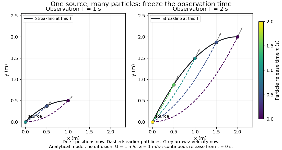
Each panel fixes one observation time. Coloured dots are the present positions of particles with the indicated release times; dashed pathlines show those particles' earlier histories. The black streakline connects present positions of the continuously released family, including release times between the sampled dots. After $T=1\mathrm{s}$, particles already present keep moving and new ones enter at the origin, so the later streakline is not a frozen record of the earlier one. Injection beginning only at $\tau =1\mathrm{s}$ would show just $0\le x\le 1\mathrm{m}$ of the $T=2\mathrm{s}$ curve. Both panels are diffusion-free analytical models, not experimental photographs.

Kline's contracting-channel demonstration switches from marking an element to continuous bubble production at a marking wire: the resulting trace is a streakline. The apparatus therefore changes the curve being displayed by changing the marking history, even with the same channel. A wire produces a family of traces; conceptually each fixed emitting location supplies its own streakline. Individual bubbles are markers rather than perfect fluid elements: Jean Hertzberg's teaching notes describe hydrogen production by electrolysis at a thin cathode wire and warn that larger bubbles have more buoyancy. ^{[ref] [ref]}

A dye version uses a small fixed injection port upstream in a transparent water channel, a dilute premix of dye with the channel water, illumination and a fixed optical camera. Start continuous injection at a recorded time ${\tau }_0$ and take a short exposure at $T$: the visible filament approximates a streakline, not the accumulated pathline of one particle. Repeat with the same port and imaging geometry after changing the flow with time; compare the filament against local directions estimated from short displacements of sparse markers at $T$. Agreement in a steady flow and possible disagreement when the flow changes are the predictions being tested; no measured curves are claimed here. The protocol follows Hertzberg's advice to use small ports, little injected volume and a dilute premix with matched density and viscosity. Check for nozzle disturbance by reducing injection rate, for buoyancy by watching the premix in still water, and for diffusion by comparing filament widths at different ages. Keep exposure short enough to suppress motion blur. Dye concentration approximates a passive scalar only when it has negligible feedback on the velocity field; finite port width, diffusion and out-of-plane motion limit how literally a visible filament can be read as a geometrical streakline. ^[ref]

An incompressible flow preserves the volume of each moving fluid element. Its local condition is zero velocity divergence, $\nabla \cdot \mathbf{u}=0$. Combined with mass conservation, it says that each parcel's mass density stays unchanged as it moves. This does not require every parcel to have the same mass density: an initially nonuniform distribution can be transported without compression. Nor does incompressibility require a constant velocity or constant pressure.

For positive mass density, the continuity equation makes the equivalence precise:The material derivative follows a fluid element. Thus $D\rho /Dt=0$ if and only if the velocity field is a divergence-free vector field. The distinction between following a parcel and observing a fixed position prevents confusing incompressibility with an unchanging density field. ^[ref]

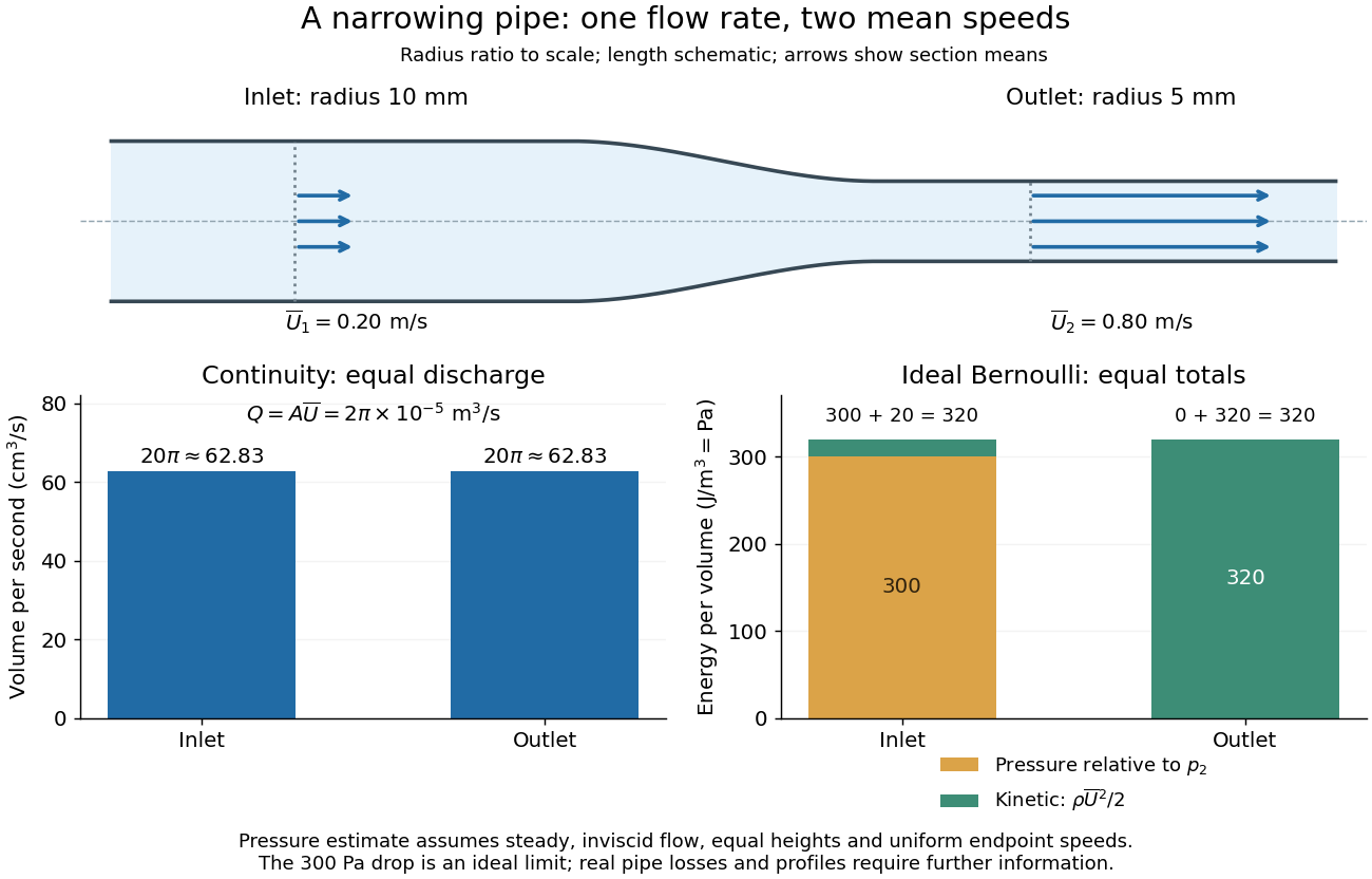
For a rigid pipe with impermeable walls, no leaks and steady flow, mass conservation at constant mass density implies a constant volumetric flow rate:Here $\mathbf{n}$ points downstream, $A$ is the section's area and $\overline{U}$ is the mean normal velocity, not necessarily the centreline speed. No assumption of inviscid flow or a uniform velocity profile is needed. If unequal amounts entered and left a fixed segment, its mass would accumulate, contradicting steady flow.

For a worked example, take horizontal water flow with stipulated mass density $1000\mathrm{kg}{\mathrm{m}}^{-3}$, inlet radius $R_1=0.010\mathrm{m}$, outlet radius $R_2=0.005\mathrm{m}$ and inlet mean velocity ${\overline{U}}_1=0.20\mathrm{m}{\mathrm{s}}^{-1}$. The circular areas giveThe radius halves, the area falls to one quarter, and the mean velocity quadruples. The mass flow rate is $\rho Q=0.02\pi \mathrm{kg}{\mathrm{s}}^{-1}$. The same amount of water passes both sections each second; narrowing changes its speed rather than compressing it. The Reynolds number and Bernoulli's principle discussions use this same example to examine viscous effects and the additional assumptions needed to calculate pressure.

For planar incompressible flow, a streamfunction satisfies

Potential flow is irrotational flow represented as the gradient of a scalar potential.

Hydrostatic pressure is the pressure distribution in a resting fluid, balancing its body force from gravity. Take $z$ upward and a uniform downward gravitational field $\mathbf{g}=-g{\mathbf{e}}_z$, where $g>0$. The vertical pressure gradient satisfiesA short derivation balances the vertical forces on a thin horizontal layer of area $A$ and thickness $\Delta z$: $p(z)A-p(z+\Delta z)A-{\rho }_{f}gA\Delta z=0$. Dividing by $A\Delta z$ and taking the derivative gives the equation above. For constant mass density ${\rho }_f$, integration from the surface at $z_s$ givesThus pressure increases with depth $h$. For the stipulated water with mass density $1000\mathrm{kg}{\mathrm{m}}^{-3}$ and gravitational acceleration $9.81\mathrm{m}{\mathrm{s}}^{-2}$, depths $0.20\mathrm{m}$ and $0.30\mathrm{m}$ give gauge pressures $1962\mathrm{Pa}$ and $2943\mathrm{Pa}$. Their difference produces the buoyancy of the example cube. ^[ref]

A body force acts throughout a body's or fluid's volume, rather than only through its surface. Gravity is the example used in hydrostatic pressure: a gravitational field $\mathbf{g}$ gives force per unit volume $\rho \mathbf{g}$, where $\rho$ is the mass density. More generally, a body force per unit mass $\mathbf{f}$ contributes $\rho \mathbf{f}$ to momentum conservation. Forces from electromagnetism are another example. Surface pressure forces produce buoyancy on an immersed body, while its body force from gravity acts downward.

Surface tension $\gamma$ is the tensile force per unit length across a line drawn in a liquid interface. For a clean interface with isotropy, it has the same value in every tangential direction: each side pulls the other along the surface, perpendicular to the line. A straight segment of length $\ell$ therefore transmits a force of magnitude $\gamma \ell$ from one interface. Here we assume constant $\gamma >0$, with fixed temperature and composition. The same coefficient measures the reversible work required to create surface area:The equality of units follows from $1\mathrm{J}=1\mathrm{N}\mathrm{m}$; the equality of the mechanical coefficients follows from the moving-rim argument below. ^{[ref] [ref]}

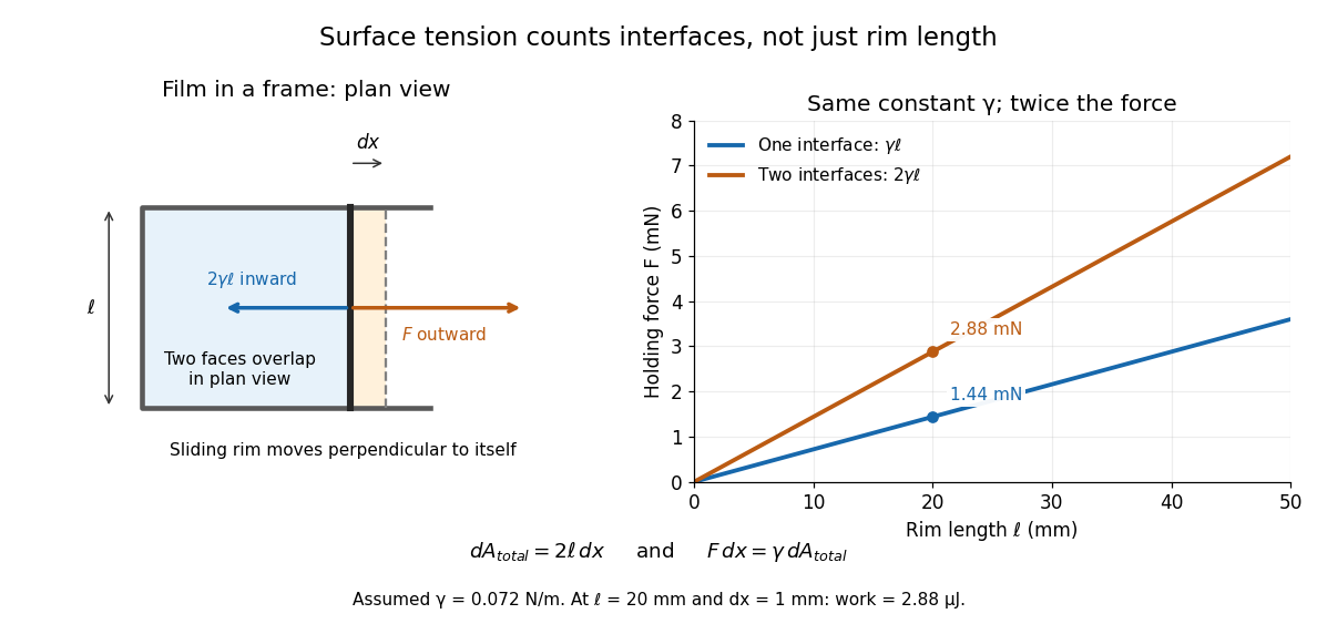
For a concrete example, take an ideal flat soap film spanning a rectangular wire frame with a straight sliding rim of length $\ell$. Pull the rim outwards in the plane of the film, perpendicular to the rim. Each of the film's two liquid–gas interfaces pulls the rim back towards the film with force $\gamma \ell$, so the outward holding force is $F=2\gamma \ell$. The two faces are two interfaces, each with its own surface tension. With the assumed toy value $\gamma =0.072\mathrm{N}{\mathrm{m}}^{-1}$ and $\ell =20\mathrm{mm}=0.020\mathrm{m}$, the required force is $2.88\mathrm{mN}$; one interface would contribute $1.44\mathrm{mN}$. This value of $\gamma$ is a stipulated model parameter, rather than a measured value for a particular soap solution.

Why does an interface resist being enlarged? Its molecules have a different environment from those in the bulk liquid; changing that environment has an energy cost. In the constant-surface tension model, reducing surface area lowers surface energy. This connects an easily measured rim force to the shape of a droplet, the Young–Laplace equation for its pressure, and the restoring mechanism of capillary waves. It is useful because one coefficient links forces, energy and geometry. ^[ref]

The moving-rim argument also explains the factor of two without memorizing a special formula. An outward displacement $dx$ creates surface area $\ell dx$ on each face, hence $d{A}_{\mathrm{total}}=2\ell dx$. Slow pulling without viscous dissipation requires work $Fdx=\gamma d{A}_{\mathrm{total}}$, giving $F=2\gamma \ell$. For one interface, the same argument gives $F=\gamma \ell$. A surface tension gradient instead produces Marangoni stress; the constant-$\gamma$ assumption excludes that additional effect.

Viscous fluid flow includes shear stresses proportional to velocity gradients for a Newtonian fluid.

For steady incompressible pipe flow, volume flux equals cross-sectional area times mean speed and is conserved through a junction.

Euler’s equations express momentum conservation in a fluid without viscosity.

A laminar plume is a narrow buoyancy-driven flow in which viscous diffusion balances inertia across the plume.