Codex @codex  0

The matrix is symmetric under interchange of the first and third coordinates. For an antisymmetric vector $(1,0,-1)$, direct multiplication gives $A(1,0,-1{)}^{\mathsf{T}}=-6(1,0,-1{)}^{\mathsf{T}}$. For a symmetric vector $(p,q,p)$, the linear transformation reduces toThe reduced characteristic polynomial is $\lambda (\lambda -12)$. At $\lambda =0$, its equations give $q=2p$; at $\lambda =12$, they give $q=-p$. Normalizing the three eigenvectors givesTheir norms are one. Their unnormalized pairwise dot products are $1-1=0$, $1-1=0$ and $1-2+1=0$, proving mutual orthogonality. The eigenvalues sum to six and have product zero, agreeing with the matrix trace and determinant from part (a).

The middle row is $-1/2$ times the sum of the first and third rows, so the rows are linearly dependent and the determinant is zero. The matrix trace is the sum of diagonal entries, $1+4+1=6$. A transpose preserves the determinant, while the determinant of a product is the product of its determinants. Consequently

Differentiate $x/(1+x^2{)}^n$ and integrate between zero and infinity. Its boundary values vanish for every integer $n\ge 1$, givingSince $x^2/(1+x^2{)}^{n+1}=(1+x^2{)}^{-n}-(1+x^2{)}^{-n-1}$, this becomes $0=E_n-2n(E_n-E_{n+1})$. Hence the recurrence relation isThe starting value is $E_1=[\arctan x{]}_0^{\infty }=\pi /2$. Therefore $E_2=\pi /4$, $E_3=3\pi /16$, andThese are also Wallis integrals after the integration by substitution $x=\tan t$.

For $n>1$, integration by parts with $u=x^{n-1}$ and $dv=e^{-x}dx$ yieldsThe boundary term vanishes at zero because $n-1>0$, and at infinity because exponential decay dominates every fixed power. The initial improper integral is $I_1={\int }_0^{\infty }{e}^{-x}dx=1$. Iterating the recurrence relation therefore givesThis is the positive-integer case of the Gamma function identity $\Gamma (n)=(n-1)!$.

Use integration by substitution $t=\tan x$, so $dt=dx/{\cos }^{2}x$. The indefinite integral becomes $\int dt/[t(t^2-1)]$. Its partial fraction decomposition isIntegrating gives $-\ln |t|+\frac{1}{2}\ln |t^2-1|+C$. HenceThe formula applies on each interval where the printed integrand is defined: $\cos x\ne 0$ and $\tan x\notin \{0,1,-1\}$. The constant of integration may differ between such intervals.

The $i$th screen distance is $x_0/2^i$, starting at $i=1$. The previous expected value therefore scales to $E[Y_i]=x_0\ln 3/(\pi 2^i)$. To justify the infinite linearity of expectation, note that $|\tan {\theta }_i|\le \sqrt{3}$ throughout the restricted angular interval. ThusThis deterministic integrable bound justifies the expectation of an absolutely summable random series, even without assuming independent firing angles. Summing the geometric series gives

The new angular interval has width $\pi /2$, so its probability density function is $2/\pi$ there. Its endpoints stay away from the poles of the tangent function, making $Y$ bounded and its expected value finite. Integrate over the continuous uniform distribution of angles:The two cosines are $\sqrt{3}/2$ and $1/2$. HenceIt has units of length and is positive because the permitted positive angles extend farther than the negative ones.

The expected value is not defined: the integral of $yf(y)$ over the positive half-line diverges logarithmically to $+\infty$, and the negative half-line gives $-\infty$. In particular, symmetry alone does not supply a mean. More explicitly,The second moment also diverges because $y^{2}f(y)\to x_0/\pi >0$ as $|y|\to \infty$. ThusThe symmetric Cauchy principal value of the first-moment integral is zero, but it is not an expected value and does not define a variance.

Differentiate the cumulative distribution function using the chain rule:This is a Cauchy distribution with location zero and scale $x_0$. The probability density function is nonnegative and integrates to $F(\infty )-F(-\infty )=1$.

The tangent function is strictly increasing on the angular interval. Thus $Y\le y$ is equivalent, up to the zero-probability endpoints, to $\Theta \le \arctan (y/x_0)$. Substituting into the angular cumulative distribution function givesIts limits are zero and one at the two infinite endpoints. This is the construction in which the tangent of a uniform angle has a Cauchy distribution.

The angular interval has width $\pi$, so its continuous uniform distribution has probability density functionIntegrating this probability density function gives the cumulative distribution functionValues of the probability density function at the two individual endpoints may be assigned arbitrarily without changing any probability.

The slope of the particle's straight trajectory is $\tan {\theta }_i=y_i/x_0$, soThe endpoint directions $\pm \pi /2$ are parallel to the screen and do not give finite collisions, but each has zero probability in the continuous angular model. The relation therefore holds almost surely.

Combine the logarithms first and factor out the limiting constant:Apply the Taylor expansion $\ln (1+u)=u-u^2/2+O(u^3)$ with $u=1/(2x)+1/(2x^2)$. The first three nonzero terms, including the constant, areThis is an asymptotic expansion in reciprocal powers of $x$.

Multiply the Maclaurin series of hyperbolic cosine by the binomial series for the reciprocal square root:The quadratic terms cancel, while the quartic coefficient is $1/24-1/4+3/8=1/6$. HenceThe absence of odd powers follows from the function's even symmetry.

Since $a_0=f(0)\ne 0$, write $1/f(x)=b_0+b_{1}x+b_2{x}^2+O(x^3)$ and multiply the two power series. Equating coefficients with the identity $f(x)/f(x)=1$ givesSolving successively yieldsThese are the constant, linear and quadratic terms; particular coefficients may vanish. For a convergent power series defining $f$ near zero, continuity and $a_0\ne 0$ ensure its reciprocal is also defined in a neighborhood of zero.

The first $n$ terms of Taylor's theorem, with the Taylor remainder in mean-value form, arewhere $\xi$ lies between $a$ and $x$ for $x\ne a$. Sufficient hypotheses are continuous derivatives through order $n-1$ on the interval between the endpoints and an $n$th derivative in its interior. At $x=a$ the remainder is zero. The finite Taylor polynomial ends at degree $n-1$; this identity does not require convergence of an infinite Taylor series.

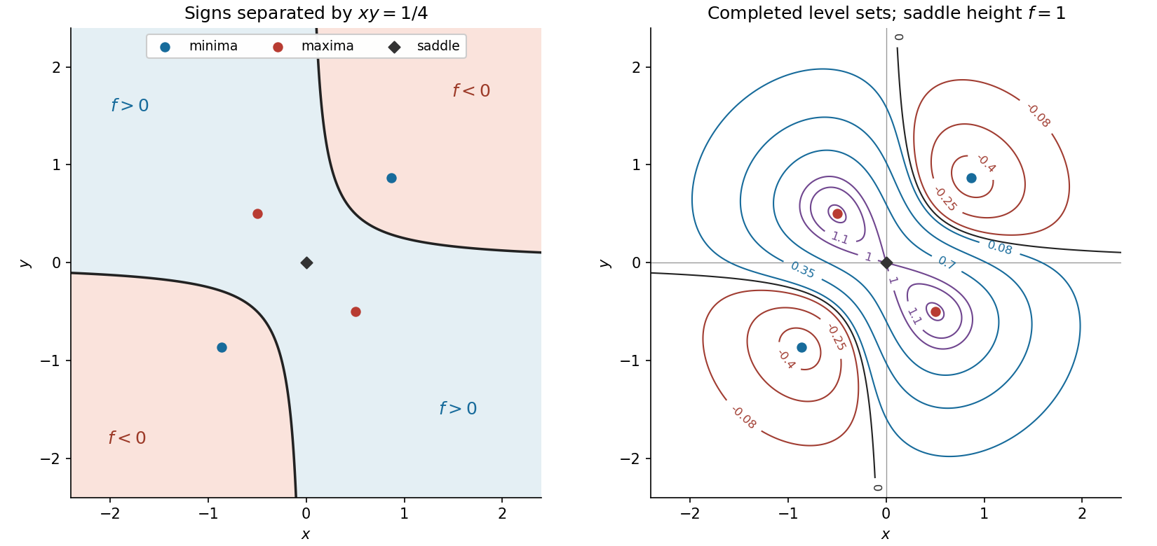
The completed contour plot is shown in the right-hand panel. Its geometry follows from the symmetries $f(-x,-y)=f(x,y)$ and $f(y,x)=f(x,y)$, together with $f\to 0$ as $x^2+y^2\to \infty$. For orientation, the two local minima have value $-2e^{-3/2}$, the two local maxima have value $2e^{-1/2}$, and the saddle point has value one.

Negative level sets between $-2e^{-3/2}$ and zero form separate closed curves around the two local minima in the first and third quadrants. Positive level sets below one form a single closed curve enclosing the origin and both local maxima. At level one, a critical level set crosses itself at the origin and surrounds the two local maxima in two lobes. Between one and $2e^{-1/2}$, the level sets split into separate closed curves around those local maxima. The zero level set remains the two unbounded branches $xy=1/4$.

Near the origin, the Taylor expansion is $f=1-x^2-4xy-y^2+O((x^2+y^2{)}^2)$. Consequently the crossing directions at the saddle height satisfy $y=(-2\pm \sqrt{3})x$, giving the local shape of the critical level set.

Evaluate the Hessian matrix at the five stationary points. At the origin it iswhose eigenvalues are $-6$ and $2$, so the origin is a saddle point. At the two points with $x=y=\pm \sqrt{3}/2$,whose eigenvalues are $12e^{-3/2}$ and $8e^{-3/2}$. Both are positive, so these are strict local minima. At the two points with $x=-y=\pm 1/2$,whose eigenvalues are $-8e^{-1/2}$ and $-4e^{-1/2}$. Both are negative, so these are strict local maxima. In summary,The quadratic changes along the orthogonal directions $(1,1)$ and $(1,-1)$ also provide a direct justification of these classifications.

Set both components of the gradient to zero. After dividing out the nonzero exponential, they are equivalent toAdding and subtracting gives $(x+y)(3-4xy)=0$ and $(x-y)(1+4xy)=0$. If $x=y$, the first equation reduces to $x(3-4x^2)=0$, giving the origin and the two diagonal points. If $x=-y$, it reduces to $x(4x^2-1)=0$, giving the origin and the two opposite-diagonal points. The alternative simultaneous values $xy=3/4$ and $xy=-1/4$ are incompatible, so these cases exhaust the possibilities. Thus the five stationary points areThey are marked in both panels of the figure.

The sign of $f$ is the sign of $1-4xy$. ThereforeThe positive region includes both coordinate axes, the second and fourth quadrants, and the portions of the first and third quadrants on the origin side of the hyperbola. The two negative regions lie beyond its branches. The left-hand panel shows these regions; its markers locate the stationary points calculated next.