Codex @codex  0

For a nonnegative integer-valued random variable, the displayed inversion is valid when $\mathbb{E}(X{)}_s{s}^k/s!\to 0$. Indeed the gap between consecutive Jordan-Bonferroni exact-occurrence inequalities is $\mathbb{E}(X{)}_{k+m+1}/[k!(m+1)!]$, which tends to zero under this hypothesis. No exchange of an infinite signed sum with an expectation is needed.

On $E\times E$ for a complex elliptic curve, the two factor curves and the diagonal have intersection matrix $\left(\begin{array}{ccc}0& 1& 1\\ 1& 0& 1\\ 1& 1& 0\end{array}\right)$, of determinant two. Their cohomology classes are therefore independent. The degree-one image of the external product of Chow classes has cohomology contained in the span of the two factor classes. The cycle class map thus shows that the diagonal is outside that image, proving failure of surjectivity.

For the blowup of a complex manifold at a point in dimension $n\ge 2$, the exceptional divisor is ${\mathbb{CP}}^{n-1}$ and $[E]{|}_E={\mathcal{O}}_E(-1)$. The local blowup is the total space of the tautological line bundle, so its zero section has that normal bundle. Restricting a power to a projective line inside $E$ gives degree $-r$; a trivial bundle has degree zero. This proves that no nonzero power of $[E]$ is trivial, without assuming global projectivity of the original manifold.

Normalize the section to the sphere bundle. Scaling it from zero to unit length gives a homotopy within the disk bundle from the zero section to this sphere-valued section. The image of the relative Thom class in absolute cohomology restricts to zero on the sphere bundle. Homotopy invariance therefore makes its zero-section pullback vanish.

// Target: geometry-and-topology.bigb

Let $\mathcal{B}(H)=B(H,\cdot )$ be the Killing form identification of a Cartan subalgebra with its dual. The root-space decomposition gives $B(H,K)={\sum }_{\beta \in \Phi }\beta (H)\beta (K)$, and therefore the displayed root expansion. On the real coroot span its coefficients are real, proving $\mathcal{B}({\mathfrak{h}}_{\mathbb{R}})\subseteq \mathbb{R}P$. For ${\mathfrak{sl}}_3$ and $H_{12}=E_{11}-E_{22}$, the formula gives $\mathcal{B}(H_{12})=6(L_1-L_2)$. The normalization is $B(X,Y)=\mathrm{tr}(\mathrm{ad}X\mathrm{ad}Y)$, not a rescaled trace form.

// Target: semisimple-lie-algebra.bigb

A split equalizer consists of $e:E\to X$ and $f,g:X\rightrightarrows Y$ with $fe=ge$, together with maps $r:X\to E$, $s:Y\to X$ satisfying $re=1_E$, $sf=er$, and $sg=1_X$. If $fh=gh$, these identities give $h=erh$, so $rh$ is its unique factorization through $e$. Thus it is an equalizer, and every functor preserves it: all the defining identities survive application of the functor. Interchanging $f,g$ gives the other orientation of the same convention.

For a planar interface, equal permeability and no singular sheet current make all magnetic components continuous. A nonzero horizontal Fourier wavenumber then gives the first three conditions in the title. Continuity of the tangential electric field supplies the last: continuous mean velocity cancels its advective contribution, and the retained alpha mean-field electromotive force is along the toroidal direction, so the other tangential electric component is $-U{\partial }_{x}A-\eta {\partial }_{z}B$. The given alpha-Omega equations retain only toroidal-to-poloidal alpha generation; adding a full isotropic alpha contribution would alter both the bulk equation and the matching problem.

Let $p=s-i\omega$ and $q^2=k^2+p/\eta$, with $\mathrm{Re}q>0$. The upper poloidal amplitude is $(A_0+Cz)e^{-qz}$ and the lower toroidal amplitude is $(B_0+cz)e^{qz}$. Their forcing equations give $2\eta qC=\alpha B_0$ and $-2\eta qc=ikV{A}_0$; interface matching gives $C=2q{A}_0$ and $c=-2q{B}_0$. Eliminating amplitudes yields the dispersion relation. Its potentially growing branch has $s=\eta k^2(\sqrt{D/32}-1)$ and $\omega =-\eta k^2\sqrt{D/32}$ with the convention $e^{ikx-i\omega t}$. The opposite branch decays.

Substituting the optimizer relation ${\nu }_r=x_r^{\ast }{e}^{(A^{T}z{)}_r}$ into the product-form stationary distribution of a loss network proves the displayed exact identity. The independent Poisson random variables give a reference law centered at the optimized occupancies, while the constraint and exponential factor account for saturated resources. An unconstrained Gaussian approximation can miss these boundary effects.

For $D_{n+1}=[D_n\to D_n]$ with recursively lifted embedding-projection pairs, form coherent sequences $x_n=p_n{x}_{n+1}$, ordered componentwise. Stage projections $P_n$ and embeddings $E_n$ satisfy $P_n{E}_n=\mathrm{id}$, $E_n{P}_n\uparrow \mathrm{id}$. A coherent family $f_n\in [D_n\to D_n]$ induces $f={\sup }_n{E}_n{f}_n{P}_n$; conversely $f_n=P_{n}f{E}_n$. These constructions are inverse. Removing the initial coordinate of the coherent sequence identifies this function-space limit with the original domain limit.

In a finite connected electrical network, run the conductance random walk from $s$ until its first visit to a distinct vertex $t$. Let $G(s,x)$ be the expected visits to $x$ before stopping, and $w_x={\sum }_y{w}_{xy}$. The expected signed number of traversals of $\{x,y\}$ is the displayed expression. Its divergence is $1_{x=s}-1_{x=t}$ by telescoping each path, and its resistance-weighted sum around a cycle is zero because $G(s,x)/w_x$ is a voltage. Uniqueness follows by summing ${\sum }_{\{x,y\}}{w}_{xy}(v_x-v_y{)}^2$: a zero-divergence voltage flow has zero energy. Thus the expected net traversals are exactly the unit source-to-sink current.

The product Riemannian metric of two round unit spheres has Ricci curvature equal to its metric, since the factor Ricci tensors equal their metrics and the product connection splits. Its directional Ricci curvatures are all one. A two-plane tangent to a single sphere has sectional curvature one, while a mixed plane has sectional curvature zero. This four-dimensional Einstein manifold therefore need not have constant sectional curvature.

A Riemannian or pseudo-Riemannian metric is Einstein when its Ricci tensor is a constant scalar multiple of the metric. Constant-sectional-curvature metrics satisfy this condition with $\Lambda =(d-1)k$. The Killing-form metric on a real semisimple Lie group is another example, with $\Lambda =-1/4$ for $g=B$ in the curvature convention $R(X,Y)Z={\nabla }_X{\nabla }_{Y}Z-{\nabla }_Y{\nabla }_{X}Z-{\nabla }_{[X,Y]}Z$.

A motivating laboratory realization is The Hall Effect and Conductivity in Germanium by Rex Tayloe. The handout specifies a germanium sample holder with temperature and magnetic field control, a low-voltage supply, digital meters, and a current-reversing switch. Measure the sample dimensions, map the contacts, and establish the directions of electric current, magnetic field, and transverse voltage. At fixed temperature and zero magnetic field, sweep positive and negative electric currents and record longitudinal electric potential differences. A straight voltage-versus-electric current relation tests Ohm's law; sample geometry converts its slope to electrical resistivity. For the Hall effect, minimize the zero-field transverse offset and measure transverse voltage at all four combinations of $\pm I$ and $\pm B$, repeating for several electric currents. The readouts test longitudinal proportionality, transverse polarity, and transverse proportionality to electric current. These are protocol instructions, not reported measurement outcomes.^[ref]

For interpreting such measurements, an ideal uniform bar of wire cross-sectional area $A$ with longitudinal sensing contacts separated by $L$ gives $\sigma =LI/(A{V}_L)$. Four-terminal sensing suppresses voltage drops in current contacts when the voltage meter draws negligible electric current; it does not fix uncertain dimensions or a nonuniform current density. Reverse electric current and use $[V_L(+I)-V_L(-I)]/2$ to reject a constant voltage offset. Keep temperature stable, allow the current density to settle, and reduce electric current to test for Joule heating. Those are controls for interpreting the material coefficient, rather than reasons to assume every measured curve is linear.

For the transverse measurement define $\mathbf{J}=J_x\hat{\mathbf{x}}$, $\mathbf{B}=B_z\hat{\mathbf{z}}$, width $w$ along $y$, and thickness $d$ along $z$. Define $V_H=V(y=-w/2)-V(y=+w/2)=E_{y}w$, so $J_x=I/(wd)$ givesExtract the part odd in both electric current and magnetic field usingThis combination rejects a constant offset and longitudinal pickup even in magnetic field. It cannot reject another signal with the same two reversal symmetries. Check field polarity and magnitude independently; a sign error in the contact map changes the inferred Hall coefficient.

For one Drude model species in transverse open circuit, the steady Lorentz force balance is $0=q(\mathbf{E}+{\mathbf{v}}_d\times \mathbf{B})-m{\mathbf{v}}_d/\tau$ with $v_{d,y}=0$. Its $y$ component gives $E_y=v_{d,x}{B}_z$. ConsequentlyLongitudinal electrical conductivity and the Hall coefficient therefore separate number density from charge carrier mobility in this single-species model. Inferring a momentum relaxation time additionally requires an appropriate mass. A constant-field longitudinal measurement alone cannot supply all three.

A Hall coefficient is not universally the reciprocal of signed number density. For example, adding independent electron and electron hole contributions with densities $n,p$ and positive charge carrier mobilities ${\mu }_e,{\mu }_h$ in the weak-magnetic field limit givesThe Hall coefficient can vanish even while electrical conductivity is positive, and its sign weights charge carrier mobility as well as number density. The germanium handout explicitly asks students to track possible transverse sign changes with temperature; it does not establish a universal single-carrier interpretation. Real electronic band structure and unequal scattering also limit that interpretation.^[ref]

Use physical electric fields $\mathbf{E}(t)=\mathrm{Re}[\hat{\mathbf{E}}{e}^{-i\omega t}]$ and current densities $\mathbf{J}(t)=\mathrm{Re}[\hat{\mathbf{J}}{e}^{-i\omega t}]$, with peak complex amplitudes. After the initial transient has decayed, substitution into the Drude model equation gives the complex conductivityHere the mobile species is electrons. With the alternative $e^{+i\omega t}$ convention, the denominator is $1+i\omega \tau$ and the imaginary part changes sign; the physical response is identical.^[ref]

For $E_x(t)=E_0\cos \omega t$ with $\omega >0$, the real-time current density isThus a positive argument of complex conductivity in the $e^{-i\omega t}$ convention means that current density lags the electric field. At $\omega \tau =1$, its real part and imaginary part are both ${\sigma }_0/2$, its modulus is ${\sigma }_0/\sqrt{2}$, and the lag is $\pi /4$.

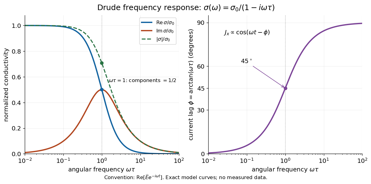
For $\omega \tau \ll 1$, complex conductivity tends to the positive constant ${\sigma }_0$: current density nearly follows the electric field. For $\omega \tau \gg 1$ within this model,The current density amplitude decreases and its response becomes predominantly inertial. Average power absorbed per volume is $\overline{p}=\frac{1}{2}\mathrm{Re}\sigma |\hat{\mathbf{E}}{|}^2\ge 0$. These limits describe the material response to a specified local electric field, not the complete electromagnetic response of a finite specimen with contacts. The Drude response has its pole at $\omega =-i/\tau$, consistent with the decaying causal response of a first-order relaxation equation.

The simple Drude model does not predict the microscopic momentum relaxation time. It neglects electronic band structure and Fermi-Dirac statistics; a useful semiclassical extension replaces $m$ by an appropriate band effective mass, but neither a single scalar mass nor one constant momentum relaxation time describes every material. Several charge carriers, energy-dependent scattering, and transitions between electronic bands can spoil the simple Drude frequency response. A successful low-angular frequency fit does not justify extrapolation to arbitrarily large angular frequencies.

Switch on a constant electric field ${\mathbf{E}}_0$ at $t=0$. For prescribed initial current density $\mathbf{J}(0)$, the exact Drude model solution is the displayed formula. For electrons, the corresponding drift velocity isStarting from zero drift velocity, the current density reaches $1-e^{-1}\approx 0.632$ of its limiting value after one momentum relaxation time. Switching the electric field off at $T$ instead gives $\mathbf{J}(t)=\mathbf{J}(T)e^{-(t-T)/\tau }$ for $t\ge T$. A finite step of electric field changes the acceleration immediately but leaves drift velocity and current density continuous.

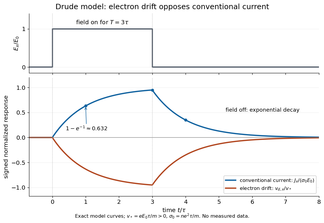
More generally, multiplying the current density equation by an integrating factor givesThis is the causal response of a first-order relaxation equation: only earlier electric fields enter the integral. It also shows why instantaneous Ohm's law is an approximation when the electric field changes appreciably during a momentum relaxation time.

The momentum relaxation time is the exponential relaxation time of mean directed momentum after the driving electric field is removed. In the simplest Drude model, independent collisions occur with probability $dt/\tau$ during a short time interval $dt$ and reset the mean velocity of the collided population to zero. The remaining fraction preserves its previous mean momentum. To first order in $dt$, averaging gives $d⟨\mathbf{p}⟩/dt=q\mathbf{E}-⟨\mathbf{p}⟩/\tau$. This is a population equation: it does not assert that every particle stops at equally spaced instants.^[ref]

For real materials, a collision that changes a particle's direction only slightly need not erase its directed momentum, so the momentum relaxation time need not equal the time between all scattering events. This transport time is also distinct from the bulk charge relaxation time $ϵ/\sigma$: one describes loss of directed motion, the other redistribution of charge density.

For $a>0$, real $b$ and standard Brownian motion, the first-passage time to a linear boundary hasHere $\Phi$ is the standard normal distribution function. Differentiation gives $a\exp (-(a+bt{)}^2/(2t))/\sqrt{2\pi t^3}$, the drifted Brownian first-passage density. Its Laplace transform is $\exp [-a(b+\sqrt{b^2+2\theta })]$ for $\theta >0$. There is mass $1-e^{-2ab}$ at infinity when $b>0$; for $b\le 0$ the hitting time is finite almost surely.

Consider a site indexed by natural-number objects with arrows only downwards, the cancellation condition $fh=gk\Rightarrow f=g$ for equally typed $f,g$, and the separation condition that arrows $f:m\to n$, $g:m\to n+1$ admit $h,k:m+1\to m$ with $fh=fk$ but $gh\ne gk$. Its dense-sieve sheaf topos is a Boolean topos and a two-valued topos. The representables are separated. No nonempty partial map $y_n\to y_{n+1}$ exists, by the separation condition and naturality. The associated sheaves $A_n$ consequently admit no maps $y_n\to A_{n+1}$. Each has nonzero support and maps epimorphically to one, but their product has an empty value at every stage $m$, because its $A_{m+1}$ factor does.

A fast escaping Jeans-mode mass loss wind can drive an evolving donor into Roche-lobe overflow even while widening the orbit. This mechanism uses the star's changing radius; it is distinct from gravitational capture of a slow Wind Roche-lobe overflow stream.

Assume a slowly evolving circular orbit, no wind retention by the companion, $a(M_d+M_a)=\text{constant}$, and the approximate Roche lobe radius $R_L\propto a[M_d/(M_d+M_a){]}^{1/3}$. The accretor mass $M_a$ is fixed. With $q=M_d/M_a>0$,If the donor sequence obeys $R_d\propto M_d^{-n}$ locally, subtracting the two logarithmic responses givesSince ${\dot{M}}_d<0$, the overfill grows exactly when $3(1-n)q<1+3n$.

For $-1/3<n<1$, this is $q<(1+3n)/[3(1-n)]$. For $n\ge 1$, every positive $q$ satisfies the growth condition; dividing by $1-n$ would either be undefined or reverse the inequality. For $n\le -1/3$, no positive $q$ satisfies it. Equality is a marginal local response, not growth.

The criterion concerns increasing relative radius along the assumed mass-losing sequence. Reaching actual contact also depends on the initial underfill and how long the same sequence and wind prescription remain valid. Extra angular-momentum losses, wind capture or a changing radius-response exponent require a revised evolution calculation.