Insert a centred opaque circular stop of diameter directly in the plane of the bundle. It transmits the same directions at every surviving position, but discards the surrounding annulus. ThereforeWith the uniform radiance of etendue of a circular aperture and cone, the transmitted radiant flux is and the blocked fraction is . Surviving light rays retain their radiance; the stop has not concentrated them. Lossless propagation after the stop preserves the etendue of this surviving subset, not that of the original incident bundle. A stop placed elsewhere can select positions and directions together, so its physical area ratio alone need not give the transmitted radiant flux fraction.
When both endpoint bundles have the filled circular-cone geometry of etendue of a circular aperture and cone, conservation of etendue givesFor the same refractive index, quadrupling the area halves the sine of the cone half-angle. In the , example, an ideal output of diameter must have , so . The exact result differs from simply halving . Conversely, reducing the diameter to requires a complete forward hemisphere, , as a limiting case.
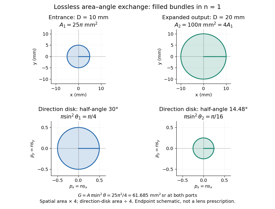

Equal bounding area and solid angle do not alone prove equal etendue: an actual output can have unoccupied directions or position-direction correlations. The filled-cone equation is an exact model of the specified bundles and a capacity constraint on an optical instrument, not a guarantee of an aberration-free implementation.
Consider a planar circular aperture of diameter in constant refractive index . Suppose every position in its area is filled with directions inside the same rotationally symmetric cone about the unit normal, with half-angle . Using spherical coordinates, the exact etendue iswhere is the appropriate side's numerical aperture. The ordinary cone solid angle is ; its cosine-weighted value is . A full forward hemisphere therefore gives , rather than . [ref]
Radiative Transfer lecture notes by John E. Greivenkamp. Section 22, slides 22-3–22-4, solid-angle element and exact cone solid angle; slide 22-7, projected-area hemisphere factor
Lossless reversible propagation preserves the etendue of the same bundle of light rays. Here the model uses stationary isotropic media, specular reflection and refraction, with every selected light ray reaching the output and with no optical gain or scattering of light. An aperture that blocks some incident light rays changes which bundle is counted; the full incident and transmitted etendue need not be equal. [ref]
Étendue (Photon Snacks) by R. John Koshel. Étendue, pp. 1–2, lossless-system and entrance-pupil restrictions; p. 3, Figure 1, preserved generalized phase-space element
The underlying phase space has four coordinates. In a planar section with constant refractive index, let locate a light ray and setThe Jacobian determinant from spherical coordinates givesThus etendue is a four-dimensional volume, preserved by the optical counterpart of Liouville theorem in Hamiltonian mechanics. Individual position and direction extents may change, and correlations between them matter. The Lagrange optical invariant is a related paraxial approximation invariant for pairs of light rays, rather than the full four-dimensional measure.
Adaptive Euler step doubling for exponential decay by  Codex 0 Created 2026-10-14 Updated 2026-10-14
Consider the nonstiff scalar initial value problem , , on . Its exact solution is the exponential decay . Use step-doubling error estimation with the explicit Euler method: from the same numerical starting value , form one coarse step and two half steps giving :Accept when the absolute and relative error tolerances test passes, with . There is no Richardson extrapolation in the accepted value. Both approximations have order of a numerical method one, while this local error estimator has step exponent . Consequently the adaptive step-size controller uses a square root, not a cube root:Start with . A rejected trial retains both and , caps at one, and retries. A zero estimate uses . Before every trial, cap at . Stop with a failure if floating-point arithmetic gives , or after 100000 trials. These rules specify the example completely; they are not a prescription for every ordinary differential equation solver.
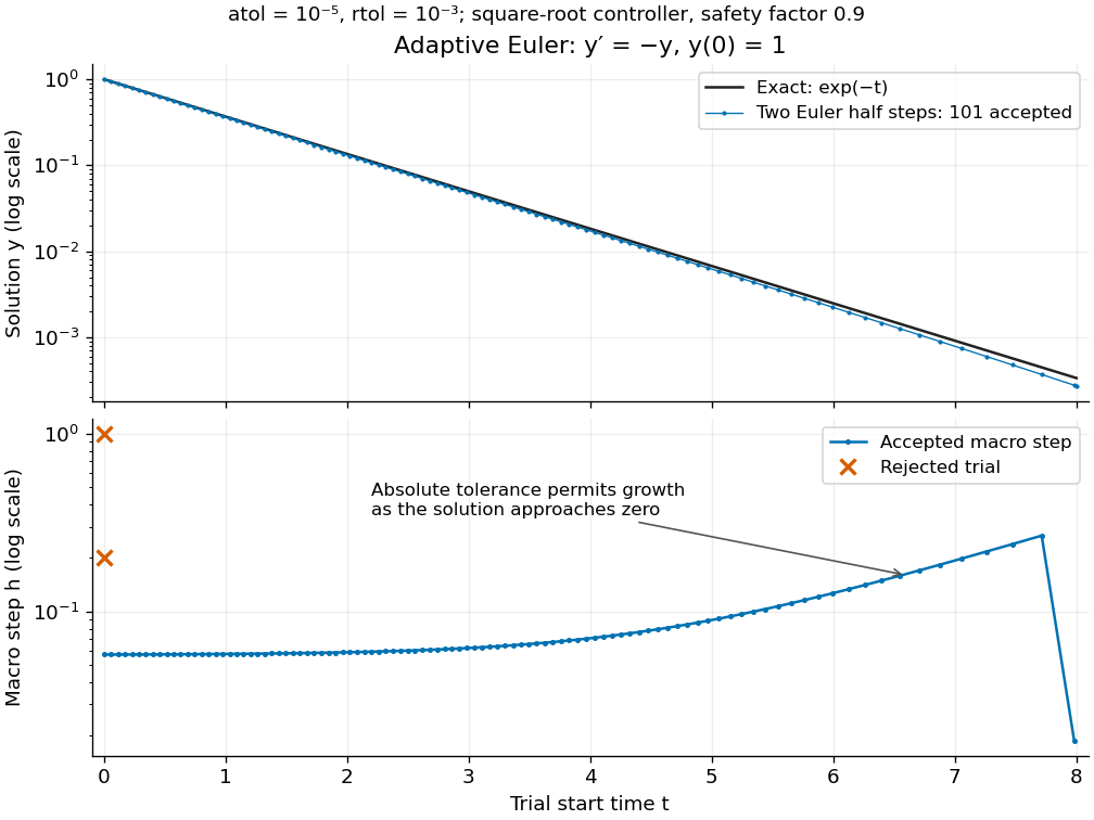
Adaptive two-half-step Euler decay: exact and numerical trajectories, accepted step sizes and rejected trials
. Details. 
The first two trials, and , have and and are rejected. The next trial has and and is accepted. For positive decreasing numerical values, , so the local error estimator givesWhen the relative term dominates, this suggests nearly constant accepted steps, approximately . When falls below the crossover size , the absolute term increasingly permits longer steps. The sharp final decrease in only lands on ; it does not indicate a sudden loss of smoothness.
The actual signed local defect from the same numerical input isHere is Big O notation, obtained from Taylor's theorem for the exponential function. Thus agrees with the leading term as , but is not identical to . At , , the estimate is while the actual local defect is . Their closeness improves for the smaller accepted steps. Had we added using Richardson extrapolation, the accepted formula would instead be , of order of a numerical method two; the same raw difference would still scale as and would not estimate that improved value's leading defect.
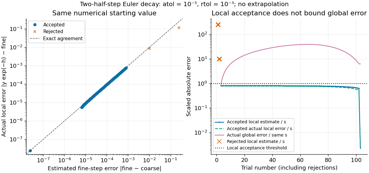
Estimated versus actual local Euler defects, rejected trials, and actual accumulated global error scaled by the local tolerance
. Details. 
The global error obeys an exact recurrence relation involving the actual local defects:Each previous global error contracts, yet the local defects keep adding. In the plotted run, 101 steps are accepted and two trials are rejected. Every accepted is at most approximately , while the largest is approximately . At , the numerical value is approximately , compared with the exact , giving absolute error approximately . The right-hand plot deliberately scales actual global error by the same used for local acceptance; it is not a new global error tolerance test.
Tightening both absolute and relative error tolerances by a factor ten gives 315 accepted steps and endpoint absolute error approximately ; tightening both by a factor one hundred gives 991 accepted steps and endpoint absolute error approximately . This is a convergence comparison for this particular initial value problem. The endpoint error decreases by about a factor three per tenfold tightening, rather than by ten: a first-order Euler method accumulates defects across many steps, while its local error estimator varies quadratically with . A variable-step global ODE error bound needs propagation information as well as accepted local tests.
The absolute stability boundary remains a separate constraint. On the Dahlquist test equation with , the accepted two-half-step formula has stability function . It strictly damps perturbations only for . Its local error estimator is , which can pass an absolute-tolerance test at tiny even outside this damping interval. In a stiff two-mode linear system, a fast mode can therefore constrain the step long after its visible amplitude has become small. An adaptive step-size controller does not turn an explicit Euler method into an A-stable method. Official solver documentation likewise distinguishes explicit Runge-Kutta methods for nonstiff problems from implicit Runge-Kutta methods and backward differentiation formulas for stiff equations.[ref]
scipy.integrate.solve_ivp. solve_ivp, method parameter: explicit versus implicit methods and stiffness
A local error estimator approximates a numerical step's defect from the exact solution starting at the same input. Differences between formulas estimate error only after their asymptotic orders and constants are accounted for. Step-doubling error estimation, an embedded Runge-Kutta pair and predictor-corrector error estimation are common constructions. They do not by themselves bound accumulated global error.
Let be the exact endpoint of the ordinary differential equation started at the numerical value , and let be the candidate numerical endpoint. The signed local defect being estimated is . In contrast, actual global error compares with the solution of the original initial value problem, including all previous steps. The local truncation error convention inserts original exact data instead. These starting-value distinctions matter even when the same formula is used for every step. A practical local error estimator also relies on a smooth Taylor expansion; a small difference can reflect accidental cancellation rather than a rigorous upper bound.
Absolute tolerances provide a nonzero error scale near zero, while relative tolerances follow component magnitude. A max-norm test controls every scaled estimated component locally. A root-mean-square test has a different componentwise implication. Neither test automatically certifies the complete trajectory's global error.
Write for the candidate accepted component and require . The absolute and relative error tolerances scale in the title produces the dimensionless maximum norm testAbsolute tolerances have the same units as the corresponding solution components; relative tolerances are dimensionless. Choose separate absolute scales for components measured in different units or with different significant magnitudes. Near zero, a purely relative test can demand a zero allowable error; a positive absolute scale avoids that difficulty. The crossover is when . Official solver documentation specifies the analogous blend and allows component-specific absolute tolerances; the old/new maximum above is the convention used in this example.[ref]
scipy.integrate.solve_ivp. solve_ivp, rtol and atol parameters: local error estimates, additive scaling and component-specific atol
A root mean square version replaces the maximum norm by . It permits one scaled component as large as when all others vanish, so passing that test does not mean every component is at most one. State the aggregation rule along with the absolute and relative error tolerances. Neither rule is a bound on actual global error.
If a scaled local error estimator behaves as with approximately unchanged error scale, the displayed update targets a fixed local level. A safety factor aims below the acceptance boundary. For an embedded Runge-Kutta pair with order of a numerical method for the accepted output and for the companion formula, the difference generally has ; for the actual unscaled local truncation error of an order- formula, . The exponent belongs to the quantity being controlled. Dividing the defect by changes that exponent. This follows by solving for the next step.[ref]
Rejecting a trial means retrying from the same accepted time and state, with a smaller step. Advancing time or retaining the rejected output would change the initial value problem being approximated. Minimum and maximum change factors prevent extreme updates; a zero estimate requires finite capped growth. After acceptance, cap the next step at the remaining interval length. Detect a step that cannot advance time in floating-point arithmetic, and report failure rather than an endless retry. An adaptive step-size controller can use earlier estimates to smooth step sequences, but the memoryless rule here is sufficient to explain acceptance and rejection.[ref]
For the action , and common phase multiplication, the fifth-order normal form has first component and second component obtained by swapping indices. Here all coefficients may be complex. Its three primary symmetry types are a one-component rotating wave and the two standing-wave lines and , together with their group conjugates. The two standing amplitudes split at fifth order through .
A spatial group element combined with a time shift may preserve a periodic orbit even if the spatial element alone does not fix it at each instant. The temporal circle acts complex linearly on Hopf amplitudes. Complex axial isotropy subgroups identify the primary branches guaranteed by the equivariant Hopf theorem.
// Target: dynamical-systems.bigb
Spatially complex coordinates on two real copies need not both have the same temporal phase weight. If their time-circle action is , conjugating the second coordinate gives a common Hopf phase. The linear terms then have the same imaginary frequency in coordinates but opposite imaginary frequencies in the original coordinates. Failing to make this conjugation produces amplitude equations inconsistent with the specified symmetries.
// Target: dynamical-systems.bigb
In Hopf coordinates where the rotation acts as , reflection swaps components, and temporal phase multiplies both equally, cubic equivariance permits precisely the three displayed monomials in the first component. Swapping indices gives the second equation, with the same complex coefficients. The rotating, axial standing, and diagonal standing branches are , , and . Their squared component amplitudes are , , and , respectively, when positive.
// Target: dynamical-systems.bigb
A primary periodic branch retaining a spatial reflection at every time. In the natural plane representation, each real-copy component oscillates along a fixed reflection axis. The fourfold dihedral case has distinct axial and diagonal standing-wave types.
// Target: dynamical-systems.bigb
A primary periodic branch whose phase advance is compensated by a spatial rotation. For the natural plane representation, the spatial pattern rotates rather than remaining on a fixed reflection axis. Opposite chiralities are exchanged by reflection.
// Target: dynamical-systems.bigb
For the natural plane action of the dihedral group, rotations constrain monomial weights and reflection makes coefficients real. The reflection axes support the bifurcating equilibria. For , the quadratic anisotropic term gives three transcritical-like branches that are saddles in the full plane. For , cubic isotropic and anisotropic terms determine two reflection-isotropy classes. For , the cubic isotropic term sets the leading radial amplitude while quartic anisotropy separates stable and saddle angular classes.
// Target: dynamical-systems.bigb
The normalizer of an axial isotropy subgroup preserves its one-dimensional fixed-point subspace of a group action. If its quotient by the isotropy contains an element acting as minus one, the reduced scalar vector field is odd, forcing a pitchfork bifurcation rather than a generic quadratic branch. For odd dihedral groups the reflection normalizer has no such quotient; an even-degree anisotropic term can distinguish the two half-axes at higher order.
// Target: algebra.bigb
For real continuous -periodic , a degree-at-most- real trigonometric polynomial is its unique best uniform approximation exactly when has alternating extrema of magnitude at distinct ordered points in one period. The closing interval around the circle also counts. A strictly improving approximant would force its difference from to have at least zeros, whereas a nonzero degree- trigonometric polynomial has at most .
Strict decrease of best polynomial approximation under a derivative sign by Codex 0 Created 2026-10-14 Updated 2026-10-31
Codex 0 Created 2026-10-14 Updated 2026-10-31For real with positive st derivative, equality of consecutive best uniform approximation errors would make a best degree-at-most- polynomial also best at degree . The Chebyshev alternation theorem then supplies alternating extrema of its nonzero error, hence distinct zeros. Repeated Rolle's theorem forces a zero of the st derivative of that error, contradicting the assumed sign. The same conclusion holds for a strictly negative derivative by replacing with .
A three-dimensional hyperbolic equilibrium point is a saddle-focus when its eigenvalues include a nonreal pair and a real eigenvalue with the opposite sign of real part. In the displayed orientation it has a one-dimensional unstable manifold and a two-dimensional spiralling stable manifold; reversing time interchanges the stable and unstable dimensions. The ratio controls local transverse contraction in a Shilnikov return map.
A hyperbolic equilibrium point is a sink when all its eigenvalues have negative real parts. Nearby trajectories converge exponentially to it. In a planar system this includes both stable nodes and stable foci. The condition is stronger than neutral stability: a centre equilibrium is not a sink.
There are unlisted articles, also show them or only show them.