Codex @codex  0

A hyperbolic equilibrium point is a source when all its eigenvalues have positive real parts. It is a sink equilibrium for the reversed flow. Every sufficiently close nonstationary trajectory leaves its neighborhood in forward time. This is distinct from an external forcing source.

The Yanai wave is the $n=0$ branch of the equatorial shallow-water dispersion relation with positive frequency:Its group velocity is $d\omega /dk=c{\omega }^2/({\omega }^2+\beta c)>0$. At low frequency it has westward phase velocity but transports energy eastward; at high frequency its phase and group velocities approach $c$.

At the critical impact parameter $b=3\sqrt{3}M$, the null orbit equation factors as $(u^{\prime }{)}^2=(u-1/3{)}^2(2u+1/3)$ for $u=M/r$. One oriented family has the displayed solution. As $\varphi \to -\infty$, positive $A$ approaches the photon sphere from larger radii and negative $A$ from smaller radii; $A=0$ is the circular orbit. The physical domain must retain $r>0$ and the positive square root in its implicit parametrization.

Quintessence models dark energy through an evolving scalar field. For a homogeneous canonical field in natural units,A positive potential dominating the kinetic term gives negative pressure. The Friedmann acceleration equation requires $w=p_{\varphi }/{\rho }_{\varphi }<-1/3$ for scalar-dominated accelerated expansion. A nonnegative canonical kinetic term prevents $w<-1$ when ${\rho }_{\varphi }>0$.

Unlike a strict cosmological constant, the field can evolve, so $w$ need not remain $-1$. This is a model class, not an identified substance.^[ref]

In A Mathematical Theory of Communication by Claude Shannon, Claude Shannon compares block uncertainty per symbol, denoted $G_N$, with conditional uncertainty given the preceding symbols, denoted $F_N$. Theorems 5 and 6 connect both decreasing approximations to the source's limiting uncertainty. He uses symbol statistics at increasing block lengths to expose structure missed by single-letter counts.^[ref] The fair marginal bits of the binary Markov source provide a small exact example of that distinction.

Consider a binary Markov source with fair initial bit and flip probability $q=1/8$. Its exact $n$-symbol information entropy is $H_n=1+(n-1)h_2(1/8)$. At $n=16$,This includes the uncertainty of the initial bit; the entropy rate itself is $h_2(1/8)\simeq 0.54356444$ bits per symbol. The finite-block difference is $(1-h_2(1/8))/n$.

For any finite block distribution, the entropy lower bound for prefix codes gives expected codeword length $L_n\ge H_n$, while Shannon coding achieves $L_n<H_n+1$. These bounds apply to each block as one source symbol, without requiring consecutive blocks to be independent. Here Huffman coding on all $2^{16}$ possible 16-symbol words gives the independently calculated value $L_{16}\simeq 9.19511361$ bits per block, or $0.57469460$ bits per symbol. The noninteger value is an expected value; each actual codeword has an integer length. As the block length grows, the prefix code bounds squeeze $L_n/n$ towards the entropy rate when an optimal code is used.

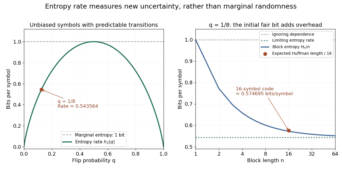
An entropy rate below one does not allow every word to fit into a shorter fixed binary word with zero error. For $0<q<1$, all $2^n$ binary words are possible, so an injective fixed-length code needs at least $n$ bits. Compression instead exploits variable codeword lengths, or the vanishing-error convention in reliable source encoding at a rate. These are different guarantees.

For a strictly stationary process on a finite alphabet, put $a_1=H(X_1)$ and $a_n=H(X_n\mid X_1,\dots ,X_{n-1})$ for $n\ge 2$. Each $a_n$ is the average remaining uncertainty in the next symbol after its history is known. More history can improve prediction, so this sequence is nonincreasing:The inequality uses conditioning reduces entropy; the last equality uses strict stationarity. Nonnegative $a_n$ therefore have a limit. By the chain rule for information entropy,The Cesàro mean converges to the same limit, proving the equality with the entropy rate. This is a statement about average information entropy. A constant almost-sure limit of the realized information content requires the further hypotheses in the Shannon-McMillan-Breiman theorem; stationarity without ergodicity in an information source explains the distinction.

Why does a gas spread through an available container? One part of the answer is counting: a nearly uniform macrostate can be realized by vastly more microstates than a macrostate with every particle crowded into one corner. Boltzmann's entropy formula turns that multiplicity into entropy. The useful insight is that a large entropy measures how many microscopic realizations fit a specified macroscopic description, rather than how untidy a picture looks.

For a specified macrostate $M$ containing $\Omega (M)$ accessible, equally likely microstates, writeHere $k_B$ is the Boltzmann constant, and $\ln$ is the natural logarithm, also written $\log$ in this article's title. The count $\Omega (M)$ is dimensionless; entropy has units of energy divided by temperature. Always specify the macrostate, the constraints and the model's microscopic resolution before counting. A microcanonical ensemble provides a familiar equilibrium setting for the equal-probability assumption. ^[ref]

The natural logarithm compresses an enormous count into a manageable number and makes products of counts into sums of entropies; see additivity of Boltzmann entropy. With this counting convention, one allowed microstate has zero Boltzmann entropy. This zero refers to the chosen model and resolution; it does not by itself assign an absolute entropy to a real material.

For unforced homogeneous incompressible flow, the vorticity equation gives $\dot{Z}=⟨{\omega }_i{\omega }_j{S}_{ij}⟩-\nu ⟨|\nabla \times \mathbf{\omega }{|}^2⟩$. Curl and full-gradient squared averages agree because the vorticity is divergence free and boundary divergences average to zero. In established high-Reynolds-number turbulence, slow integral-time evolution makes production and destruction nearly balance.

For deterministic nested partitions with mesh tending to zero, lift the polygonal interpolation of Brownian motion by its ordinary iterated integrals. These path signatures converge almost surely to enhanced Brownian motion in every Hölder rough-path metric of exponent below $1/2$, hence in $p$-variation for $p>2$. Conditioning on the partition values gives a nested martingale for the first level and the off-diagonal second levels. Moment bounds and interpolation upgrade pointwise convergence to convergence in the rough path metric.

For $2<p<3$, the support of a measure of enhanced Brownian motion is the rough-path closure of path signatures of paths in the Cameron-Martin space of Wiener measure. Polygonal convergence gives one inclusion. For the reverse inclusion, decompose Brownian motion into its polygonal interpolation and independent pinned bridges. The bridge enhancement becomes small in probability as the mesh decreases, while every finite-dimensional neighborhood of the polygonal vertices has positive Gaussian probability. Rough path translation then gives positive probability in every ball around a prescribed control path signature.

For every $2<p<3$ and every positive radius, the canonical Brownian enhancement has positive probability of lying in the displayed rough path metric ball. This controls both displacement and area. Together with Cameron-Martin quasi-invariance of enhanced Brownian motion, it puts every lifted Cameron-Martin control in the support of enhanced Brownian motion.

Rest mass is the invariant mass $m$ in the relativistic energy-momentum relation. It equals the energy measured in the particle's rest frame divided by $c^2$.

The semidiscrete system $U^{\prime }=D_{xx}U+\alpha D_{0}U$, for real fixed $\alpha$, is contractive in the periodic discrete L2 norm. Discrete summation by parts makes the drift term's real energy contribution zero and the diffusion term nonpositive. Equivalently its Fourier amplification symbol generator has real part $-4h^{-2}{\sin }^2(\theta /2)$. This continuous-time estimate does not prove stability of an arbitrarily chosen time integrator.

For zero endpoint values and real constant drift, integration by parts gives $\frac{1}{2}d\Vert u{\Vert }_{L^2}^2/dt=-\Vert u_x{\Vert }_{L^2}^2$. The drift contributes only a zero boundary term in the real part. Thus the solution is contractive, uniformly in the drift. Multiplication by $e^{\kappa x}$ converts the equation to a heat equation with constant killing rate ${\kappa }^2$, providing existence and uniqueness as well as the direct energy estimate.

The inertial range lies between the energy-containing and viscous scales. Direct forcing and viscous dissipation are small there, and nonlinear transfer carries an approximately constant mean energy flux in a three-dimensional forward cascade. Scale similarity and universality are additional statistical hypotheses.

The dissipation range contains scales at which kinematic viscosity appreciably affects velocity gradients and converts kinetic energy into heat. In a high-Reynolds-number three-dimensional cascade its characteristic length and time are the Kolmogorov microscales. Intense vortex cores can be intermittent within this range.

The equilibrium range consists of scales below the energy-containing motions whose statistics can adjust rapidly to the local energy supply. It includes the inertial range and dissipative scales. Approximate equilibrium concerns mean transfer and viscous dissipation, not absence of intermittent spatial fluctuations.

Kolmogorov 1941 theory assumes locally universal small-scale velocity statistics set by mean viscous dissipation and kinematic viscosity at large Reynolds number. In its inertial range dimensional form, $S_p(r)\sim {ϵ}^{p/3}{r}^{p/3}$. Large-scale modulation and internal intermittency require qualifying this unconditional scaling.

The Townsend-Betchov cascade cartoon organizes inertial range vorticity into sheets by bi-axial strain, then uses sheet instability and roll-up to generate finer vortex tubes. Dissipative tube cores balance stretching with kinematic viscosity. Such differing mechanisms across scales challenge literal identical-step, memoryless cascade models without contradicting a mean energy flux.