Codex @codex  0

Bulk viscosity is the dissipative response to a fluid's volume expansion or compression, distinct from the shear response. For a Newtonian isotropic fluid its isotropic dissipative stress includes ${\zeta }_B(\nabla \cdot \mathbf{v})I$, and nonnegative ${\zeta }_B$ gives nonnegative compression-related dissipation. A condensate's relative-density-flow bulk coefficient must be identified from its particular hydrodynamic equation; it is not automatically numerically identical to a dimensional Newtonian viscosity.

A uniform flow has the same velocity at every position. A constant velocity field has zero divergence and zero vorticity; a velocity potential is $\varphi (\mathbf{x})=\mathbf{U}\cdot \mathbf{x}$. It describes the remote ambient flow in idealized obstacle and line vortex problems.

An airfoil (British spelling: aerofoil) is the cross-sectional profile of a lifting surface, such as a wing or blade. Its chord is the straight segment from leading edge to trailing edge, with length $c$; its mean camber line runs midway between its upper and lower surfaces, and its thickness measures their separation. Camber is the departure of that mean line from the chord. The angle of attack describes the profile's orientation relative to the incoming flow. These independent choices let a designer alter the distribution of pressure, lift and drag, rather than simply enlarging the surface. ^[ref]

The distinction between an airfoil and a finite wing matters. A two-dimensional section model assumes no variation along span and predicts lift per unit span $L^{\prime }$. A wing of span $b$ has a spanwise distribution $L^{\prime }(z)$ and total lift $L={\int }_{-b/2}^{b/2}{L}^{\prime }(z)dz$. Its tip flow and trailing vortices generate a downward induced velocity, called downwash, which changes the local flow seen by the sections. Thus one cannot generally multiply the isolated two-dimensional $L^{\prime }$ by $b$. The wing aspect ratio $b^2/S$ measures its span relative to its reference area and helps characterize these three-dimensional effects. ^[ref]

For a thin section with small camber slopes and small angle of attack, thin airfoil theory predictswhere both angles are in radians and ${\alpha }_{L=0}$ is the zero-lift angle of attack. The model assumes two-dimensional, steady flow, incompressible flow, inviscid flow, an attached outer flow, and smooth departure at a sharp trailing edge (the Kutta condition). This last condition selects the circulation used by the Kutta–Joukowski theorem; with counterclockwise circulation $\Gamma$ positive and ${\mathbf{U}}_{\infty }=U_{\infty }{\mathbf{e}}_x$, that theorem gives $L^{\prime }=-{\rho }_{\infty }{U}_{\infty }\Gamma$ for positive lift towards $+{\mathbf{e}}_y$. The beauty is that a detailed velocity field collapses to a simple force law, while the geometry enters through ${\alpha }_{L=0}$. ^{[ref] [ref]}

A symmetric airfoil has ${\alpha }_{L=0}=0$ in this model: at $\alpha =4{}^{\circ }=\pi /45$ the predicted lift coefficient is $c_l\simeq 0.439$, and reversing $\alpha$ reverses lift. A stipulated cambered section with ${\alpha }_{L=0}=-2{}^{\circ }$ instead predicts $c_l\simeq 0.219$ at zero angle of attack. These are ideal calculations, not measurements or guarantees for a particular profile. Air parcels on the upper and lower surfaces have no obligation to arrive together at the trailing edge; the pressure and velocity field must satisfy the flow problem. A symmetric lifting section already makes an unequal-path-length explanation inadequate. ^[ref]

Real airfoils have a viscous boundary layer, even when inviscid flow approximates the outer motion. At sufficiently demanding incidence, flow separation can become extensive and the lift coefficient departs from its approximately linear law, reaches a maximum and may fall: this is aerodynamic stall. Lift does not generally vanish at aerodynamic stall. The onset depends on profile, Reynolds number, surface condition and motion history; $2\pi (\alpha -{\alpha }_{L=0})$ predicts neither a universal stall angle nor post-stall behavior. The pressure/balance experiment in lift makes this limit observable by measuring changes in the surface pressure distribution alongside the total force. ^[ref]

A wind tunnel produces controlled flow past a stationary test object. A typical arrangement uses a driving fan or pressure source, a flow-conditioning region, a test section and a downstream return or exhaust path. The stationary model makes repeated measurements of pressure, lift and drag easier while the incoming flow is controlled.

Matching a geometric shape alone does not guarantee similarity to the full-size flow. Reynolds number, Mach number, surface condition and incoming fluctuations can influence the result. The model can also block part of the test-section area, changing the flow being measured. An experiment therefore records upstream conditions and varies the relevant controls rather than treating one force reading as universal. A Pitot-static tube estimates local speed under its appropriate assumptions, while pressure ports and a force balance probe complementary aspects of the loading.

Ideal steady flow with incompressible flow, inviscid flow and irrotational flow can predict zero drag on a body that has nonzero drag in a real fluid. The zero-circulation cylinder pressure coefficient distribution gives an explicit cancellation example; viscosity and flow separation are absent from that model.

An instrument converting pressure or a pressure difference into a measurable signal. Its zero and scale must be checked separately, as illustrated by differential-pressure calibration.

An instrument for measuring pressure relative to another pressure. A liquid-column manometer uses hydrostatic pressure; a digital manometer uses a pressure transducer.

The appeal of a liquid-column manometer is that a pressure measurement becomes a visible length measurement: mass density and gravitational acceleration supply the conversion. It can compare two pressure tappings in a flowing fluid, even though the measuring liquid itself must settle into hydrostatic equilibrium. The reference connection determines which pressure difference is being measured.

The local fluid pressure, distinguished from dynamic pressure and stagnation pressure. "Static" does not require the fluid to be stationary.

Lift is the component of the fluid force perpendicular to the far-field flow relative to the body. It need not point vertically: a tilted flow changes the lift direction, and a banked wing can produce a sideways component. In a planar problem choose a unit vector ${\mathbf{e}}_D$ along the incoming relative velocity ${\mathbf{U}}_{\infty }$ and a perpendicular unit vector ${\mathbf{e}}_L$ pointing towards the chosen positive-lift side. ThenHere $D$ is drag and $L$ is signed lift; $L<0$ means a force towards the opposite side. In three dimensions the plane perpendicular to ${\mathbf{U}}_{\infty }$ also admits a separate side-force direction, so a lift axis must be specified. Lift is also distinct from buoyancy, which can exist without a relative flow. ^[ref]

The force comes from adding local surface tractions, rather than assigning a single pressure to each side. Let $\Sigma$ be the wetted body surface and $\mathbf{n}$ its unit normal vector pointing out of the body into the fluid. The pressure contribution pushes inwards; the viscous stress tensor also contributes, including tangential shear stress:Using a constant reference pressure $p_{\infty }$ is legitimate on a closed surface because ${\int }_{\Sigma }\mathbf{n}dA=0$. This surface integral makes the direction explicit: a surface-normal force is generally neither pure lift nor pure drag. Pressure and skin shear stress both enter the resultant, although the pressure term usually dominates lift on an airfoil. ^[ref]

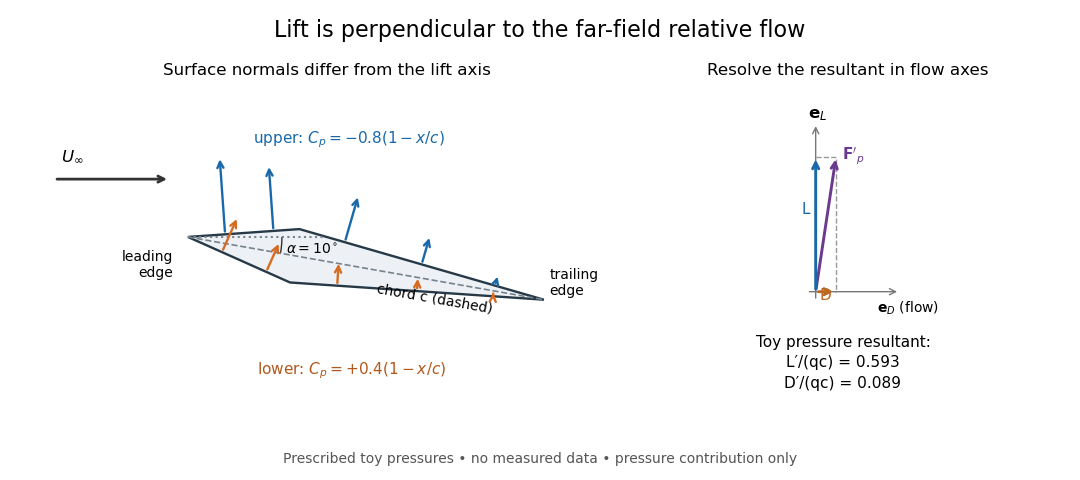
The lift coefficient isolates a useful scale. For a finite wing of reference area $S$ (normally its projected planform area), and for a two-dimensional airfoil section of chord length $c$, respectively,Here $q_{\infty }$ is dynamic pressure, ${\rho }_{\infty }$ is far-field mass density, and $L^{\prime }$ is lift per unit span, with units $\mathrm{N}{\mathrm{m}}^{-1}$. The signs of $C_L$ and $c_l$ follow the chosen lift axis. For stipulated values ${\rho }_{\infty }=1.20\mathrm{kg}{\mathrm{m}}^{-3}$, $U_{\infty }=20\mathrm{m}{\mathrm{s}}^{-1}$, $S=0.50{\mathrm{m}}^2$ and $C_L=0.60$, $q_{\infty }=240\mathrm{Pa}$ and $L=72\mathrm{N}$. Doubling $U_{\infty }$ gives four times the lift only if $C_L$ stays fixed: changes in Reynolds number, Mach number, surface condition or angle of attack can change it. ^[ref]

A motivating experiment is to compare two independently observed quantities: the lift registered by a force balance, and the lift inferred from surface pressures. A low-speed wind tunnel holds the model fixed while air passes it at adjustable speed; a calibrated balance measures forces, while small flush holes on both surfaces connect by tubing to differential-pressure sensors referenced to $p_{\infty }$. Iowa State's GA(W)-1 teaching model has $43$ taps around a $101\mathrm{mm}$ chord; its instructions give their coordinates and close the contour by repeating the first tap. A classroom comparison can combine this pressure-panel method with a balance on the same model; this is an experiment design, not a claim that those instructions report a combined measurement. ^{[ref] [ref]}

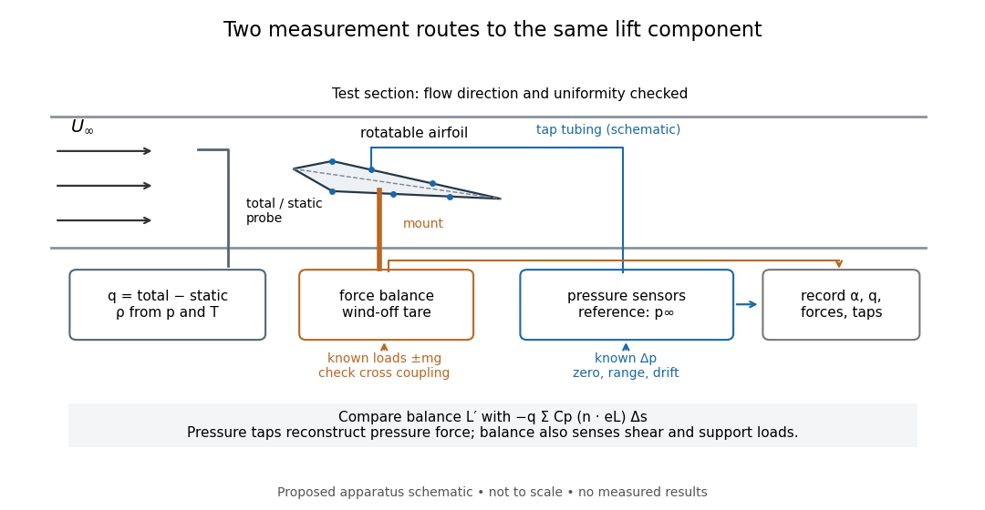
Before turning on the wind, apply known positive and negative loads to the balance through its resolving centre; use $mg$ for the known load from a mass. Record all balance channels during loading and unloading, including response to drag and torque loads, to detect cross coupling, hysteresis and zero drift. Record a wind-off tare at each model orientation so its gravitational weight does not become an aerodynamic lift reading. Map tunnel flow direction and uniformity, rather than using the fan setting as a speed measurement. Covert's MIT guide describes these calibration, tare and flow-survey requirements. ^[ref]

For each pressure channel, apply zero and several known pressure differences spanning the expected range; determine the voltage-to-pressure relation and recheck it after a run. Inspect tubing for leaks and blocked taps, and wait for readings to settle before averaging: tubing can delay a pressure signal. This calibration principle is used in NASA's electronically scanned pressure systems, where several applied calibration pressures determine each sensor's response and repeated calibration tracks drift. A simple pressure standard can instead use a liquid-column height difference and the hydrostatic pressure law. ^[ref]

Measure far-field static and total pressure outside the model's fluid wake; in low-speed incompressible flow their difference gives $q_{\infty }$ by the Bernoulli equation, so $U_{\infty }=\sqrt{2q_{\infty }/{\rho }_{\infty }}$. Record temperature and ambient pressure to determine mass density using the ideal gas law. At fixed $q_{\infty }$, step the angle of attack, repeat selected settings, and sweep back down to check reproducibility. Record balance lift, each tap's mean pressure, and fluctuation sizes. NASA describes pressure probes connected to differential transducers and emphasizes recording their reference pressure. ^[ref]

Convert each tap to a pressure coefficient $C_{p,i}=(p_i-p_{\infty })/q_{\infty }$. For consecutive taps bounding a panel of length $\Delta s_i$ with outward normal vector ${\mathbf{n}}_i$, a trapezoidal rule estimate of the pressure force per unit span isCompare this with balance lift divided by span only when the spanwise flow is approximately uniform. Agreement tests the pressure-resultant picture; disagreement calls for checking unresolved leading-edge pressure variations, skin shear stress, support loads and three-dimensional end effects before rejecting it. A force balance senses the total load, while taps alone reconstruct the pressure part. Tunnel walls and model blockage alter the effective flow and require corrections; end plates or a model extending between walls approximate two-dimensional flow but do not guarantee it. Record the Reynolds number and Mach number with the result, and do not interpret tunnel lift coefficients as universal wing data. ^{[ref] [ref]}

The Strouhal number compares the advective time $h/U$ with a prescribed forcing time $1/\omega$. Some conventions use ordinary frequency instead of angular frequency, introducing a factor $2\pi$. For a longitudinal disturbance extending over length $\lambda h$, the relevant ratio is $\lambda St$ rather than $St$ alone.

The void fraction is the fraction of a mixture's local volume occupied by gas. For a horizontally uniform bubbly liquid it is the transported concentration in a one-dimensional gas-volume continuity equation. It is distinct from gas mass fraction because gas and liquid have different mass densities.

Laminar flow is a regime of fluid flow in which the motion remains organized, with neighboring fluid parcels following smooth, coherent paths rather than the irregular interacting fluctuations characteristic of turbulence. In a straight pipe, the simplest example consists of coaxial layers sliding past one another. This describes the character of the motion, not a requirement that every parcel have the same velocity. Nor does it require steady flow: a smooth profile can evolve in time as viscosity transmits motion from a newly moving wall into a resting fluid. The unsteady wall-driven solution provides an explicit example. ^[ref]

The Reynolds pipe-and-dye experiment makes this distinction visible. A thin injected dye band can remain coherent in laminar flow, whereas irregular motion can fold it and carry dye across the pipe. However, molecular diffusion can spread dye even in laminar flow, and an inlet disturbance can move a coherent band without producing turbulence. A dye band is a streakline, not a measurement of the entire velocity field; in steady flow an ideal passive tracer's streakline coincides with a streamline. Reynolds explicitly distinguished a wandering band from one broken into eddies. ^[ref]

For a circular pipe of internal diameter $D$, define the mean axial velocity $U$ using the volumetric flow rate $Q$ and cross-sectional area $A$:Here $\rho$ is mass density, $\mu$ is dynamic viscosity and $\nu =\mu /\rho$ is kinematic viscosity. This particular Reynolds number uses the diameter and mean velocity, not the radius or centreline velocity. Small Reynolds number generally favors laminar flow, but a single universal critical Reynolds number does not distinguish it from turbulence in all geometries and experiments. Even in a given pipe, inlet conditions and the magnitude of disturbances affect the observed onset. Reynolds demonstrated this dependence by deliberately inserting a wire coil. ^[ref]

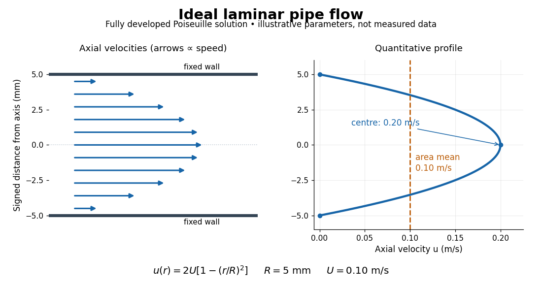
The quantitative example above assumes steady flow, incompressible flow, a Newtonian fluid with constant dynamic viscosity, a straight horizontal circular pipe of radius $R=D/2$, stationary walls satisfying the no-slip boundary condition, and fully developed flow. The last assumption means that the axial velocity profile no longer changes downstream. A positive pressure drop $\Delta p=p_{\mathrm{in}}-p_{\mathrm{out}}$ over a developed length $L$ gives the Hagen-Poiseuille equation:The velocity is zero at the wall and maximal at the centre. Averaging over the circular area, whose annuli have area $2\pi rdr$, gives $U=u(0)/2$; averaging along one diameter would give a different answer. These assumptions produce a parabola, rather than every laminar flow having a parabolic profile. ^[ref]

As a stipulated calculation, take $D=0.010\mathrm{m}$, $U=0.10\mathrm{m}{\mathrm{s}}^{-1}$, $\rho =1000\mathrm{kg}{\mathrm{m}}^{-3}$, $\mu =0.0010\mathrm{Pa}\mathrm{s}$ and $L=1.0\mathrm{m}$, and assume the developed laminar flow above. Then $\nu =10^{-6}{\mathrm{m}}^2{\mathrm{s}}^{-1}$, ${\mathrm{Re}}_D=1000$, $u(0)=0.20\mathrm{m}{\mathrm{s}}^{-1}$, $Q=7.85\times 10^{-6}{\mathrm{m}}^3{\mathrm{s}}^{-1}$ (about $0.471\mathrm{L}\mathrm{mi}{\mathrm{n}}^{-1}$), and $\Delta p=32\mu LU/D^2=32\mathrm{Pa}$. These are predictions from chosen parameters, not measurements or a claim that ${\mathrm{Re}}_D=1000$ guarantees laminar flow in every apparatus.

The beauty of this example is that a spatially varying velocity field still gives an exact relation between two accessible measurements, pressure drop and volumetric flow rate. It predicts the hydraulic resistance $\Delta p/Q=8\mu L/(\pi R^4)$. Doubling the radius therefore multiplies $Q$ by sixteen at fixed pressure drop, length and dynamic viscosity, provided the model remains applicable. This makes the laminar flow model useful for sizing narrow tubes or determining dynamic viscosity. It also explains why a persistent narrow dye band can be informative without implying that the fluid is moving as a uniform plug.

An inode is a data structure describing an object in an inode-based file system. For an ordinary file, it records file metadata such as type, owner, access permissions, size and hard link count, together with information locating the contents. In the direct-reference toy layout, inode 42 points to file data blocks 7 and 9; its two names a and b live in directory entries. Other file systems can locate contents differently, so the diagram is a model of the separation rather than a universal storage layout. ^[ref]

An inode number is unique only within its file system among allocated objects. Two different file systems can each have inode 42, referring to unrelated files. POSIX exposes the file system's device identity as st_dev and the file's serial number as st_ino; the pair identifies a file within a running system. Neither the bare inode number nor that pair is a permanent historical identifier: after reclamation, a later file can reuse the number. In particular, comparing an old saved number with a new one does not establish continuity of the file. ^[ref]

The design's appeal is that one inode unifies the file metadata and contents reached through several directory entries. Ritchie and Thompson's original 1974 account explicitly describes a directory entry as a name and an i-number, with the corresponding inode holding ownership, protection, size, content addresses and the hard link count. It gives a concrete early explanation of how names and file identity can evolve separately. ^[ref]

// Target: computer-science.bigb

NTFS is a filesystem used by Windows, organizing file metadata through a master file table and supporting features including access control lists, sparse files, named streams and metadata journaling. The metadata journal helps recover filesystem structural consistency after an interrupted operation; it does not make every application's recent data automatically durable. Files can use multiple allocation extents, and the logical byte sequence is separate from its physical placement. Exact limits and feature availability depend on the system version and configuration.^[ref]

// Target: computer-science.bigb

The File Allocation Table filesystem family tracks file storage through a table indexed by allocation cluster. A file's directory entry points to its first cluster; table entries link later clusters or mark the end of its chain. Following that chain reconstructs a fragmented file. This simple organization differs from an extent tree that describes long contiguous runs at once. FAT variants differ in entry widths and other layout rules. File length and cluster-chain traversal must agree with the on-disk metadata; the file's bytes do not necessarily occupy one contiguous interval.

// Target: computer-science.bigb

An access control list associates an object with entries describing permissions for specified users, access-control groups or principals. A file ACL might grant one access-control group read access and one user write access while denying others. The effect of multiple entries, inherited entries and defaults depends on the system's evaluation rules; treating every ACL as a simple unordered union of grants can be wrong. An ACL describes policy associated with an object, while an access check evaluates that policy for a particular operation and security context.

// Target: computer-science.bigb

A separately retained copy intended to recover files after loss or unwanted changes. A journal can be overwritten after a journal checkpoint and can faithfully commit an unwanted deletion; it does not supply that historical copy or protect against loss of the device holding the only copy.

// Target: computer-science.bigb

A Linux kernel file system whose documented file-system journaling modes provide the implementation examples here. The diagrams specify a simpler abstract protocol, not its full on-storage format.

A write whose durable result after a crash is either the complete old record or the complete new record. Its unit and failure conditions must be stated. The diagrams assume this property for each payload record, final-location record, commit marker and retirement marker; they do not derive it from the size of a file data block.