By Wissam Raji.
Cited passages: Wissam Raji, Elementary Number Theory, Section 7.2, definitions of theta and psi; Wissam Raji, Elementary Number Theory, Section 7.2, finite theta decomposition and Exercise 1.
Bond polarization is unequal sharing of electron density across a chemical bond. An electronegativity difference is a heuristic for its direction and tendency, not a unique partial atomic charge.
A simple two-site model makes the notation explicit. Represent each site by effective positive electric charge , and allocate expected electron populations to and to , with . Here is the elementary charge; these effective sites omit the internal structure of real chemical atoms. Subtraction givesFor the stipulated illustration , the populations are and , and the effective partial atomic charges are and . Fractional expected populations do not split an individual electron into pieces. The total population remains two, and the pair remains neutral. No formula connecting to has been assumed; many electron density distributions and partitioning conventions can share one qualitative electronegativity ordering.
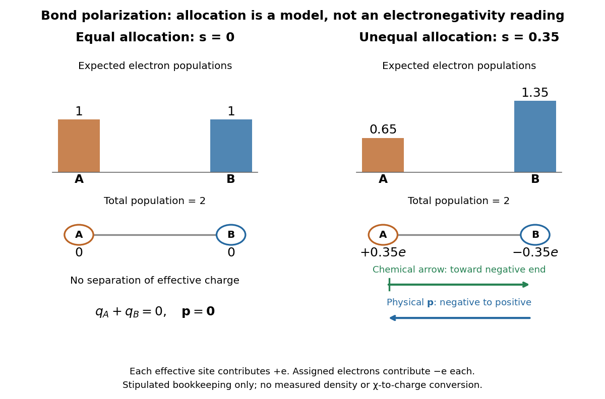
Stipulated two-site bond polarization: expected electron populations, effective partial atomic charges, and opposite chemical and physical arrow conventions
. Original model with and , effective positive site charges , and two expected electrons in total. The population bars are bookkeeping weights, not a measured electron density map. Arrow lengths illustrate direction only; no empirical electronegativity values or charge calibration are implied. Details.
A permanent electric dipole moment gives evidence of separated positive and negative electric charge in an overall neutral molecule. This is a more direct probe of chemical polarity than an electronegativity table. For hydrogen chloride, NIST lists about debye for the lowest vibrational state and debye for the equilibrium value. They describe different averaging conventions, not two contradictory measurements. The NIST WebBook traces the vibrational value debye to molecular-beam electric-resonance measurements in 1970.[ref][ref]
How does molecular beam electric resonance reveal an electric dipole moment? A source and apertures form a beam of molecules in vacuum. A first nonuniform electric field, A, selects quantum states through their different Stark effects. In a central region, C, electrodes supply a nearly uniform electric field and applied radiation drives transitions at selected frequencies. A second nonuniform electric field, B, analyzes the outgoing quantum states; a detector measures the rate of arriving molecules. In a transmission-loss arrangement, resonant radiation transfers some molecules to a quantum state rejected by B, so the measured arrival rate dips. The observable is a change in detected molecules as the radiation frequency is scanned, rather than light absorption itself. This general apparatus description is documented in a later experimental thesis; it is not a reconstruction of the exact 1970 HCl instrument.[ref]
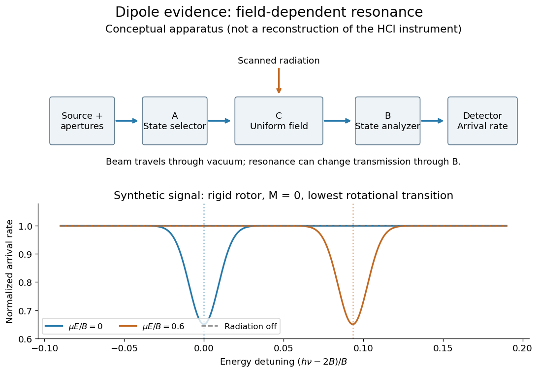
Molecular beam electric resonance: schematic state selection and a synthetic Stark effect signal from a rigid rotor model; neither apparatus dimensions nor signal curves are measured HCl data
. Details. 
The inference comes from how transition frequencies change with the known electric field. The interaction couples the electric dipole moment to the electric field; fitting the quantum mechanics of the relevant rotational states extracts its magnitude. A free rotating molecule need not show a first-order shift proportional to : the weak-field Stark effect can be quadratic. The diagram uses a simplified rigid rotor, with an energy constant, to illustrate this behavior. It omits the fine details of actual spectra.
Useful controls include scans with the radiation off to measure the baseline arrival rate, repeated scans at several calibrated electric fields, and agreement between independently assigned transitions. These are methodological checks, not claims about undocumented steps of the 1970 experiment. Field calibration and state assignment limit the inferred electric dipole moment. The published 1970 abstract confirms analysis of HCl and DCl beam-resonance spectra and combination with infrared spectroscopy intensities to obtain a distance-dependent electric dipole moment; its full apparatus and calibration record were unavailable here.[ref]
Dipole Moment and Hyperfine Parameters of H35Cl and D35Cl by E. W. Kaiser. pp. 1686–1703, authored abstract; full text unavailable
Even an accurately measured electric dipole moment is not an absolute partial atomic charge. Replacing a hydrogen chloride molecule by two point electric charges separated by bond length gives . Using debye and gives times the elementary electric charge. This is an effective two-point model, combining a vibrationally averaged electric dipole moment with an equilibrium bond length, not a unique partition of the actual electron density or a measured “18.1 percent ionic bond”.[ref]
For a molecule with several chemical bonds, molecular geometry can cancel opposing contributions to the total electric dipole moment. Carbon dioxide illustrates why an overall nonpolar molecule need not have unpolarized individual chemical bonds. An electronegativity comparison helps anticipate local bond polarization; the measured molecular electric dipole moment tests the entire electric charge distribution.
Chemical environment dependence of electronegativity by  Codex 0 Created 2026-10-13 Updated 2026-10-20
A tabulated electronegativity is useful because it compresses many comparisons, but one number per chemical element suppresses chemical context. Changing the bonded partners, bond length or electron configuration changes the conditions under which a chemical atom attracts electron density. The bond-dissociation energy can change for reasons beyond bond polarization, so attributing every extra unit of energy solely to an electronegativity difference is an approximation.[ref]
Energy Electronegativity and Chemical Bonding by Stepan S. Batsanov. §2.2, opening paragraph: bond distance and atomic valence affect bond energy
An oxidation state labels a formal allocation of electrons; it is not a measured partial atomic charge. State-sensitive electronegativity models may give different values for different oxidation states or electron configurations, while a simple chemical element table intentionally provides a common comparison convention. Likewise, replacing an isolated chemical atom by a site in an ionic crystal introduces a surrounding electric field and many neighbours. Applying the same tabulated electronegativity without adjustment becomes an additional assumption.[ref]
For the ground-state Mulliken scale, the state dependence is visible directly in the formula. Replacing by replaces with as the removal cost, and replaces with as the attachment release. These are different ionization energies and electron affinities. This isolated-ion arithmetic does not claim that a bonded chemical atom with the same formal oxidation state is an isolated ion. In a molecule, the actual electron density and dipole evidence for bond polarization supply complementary information about that environment.
The contrast between Pauling electronegativity and Mulliken electronegativity becomes clearer by following the measurements into the formulas. A Pauling bond-energy excess compares three compatible bond-dissociation energies; Mulliken electronegativity takes the arithmetic mean of an ionization energy and an electron affinity. The former asks how much stronger an unlike-atom chemical bond is than a stipulated baseline; the latter combines two different isolated-species energy gaps.
Actual readouts precede those model choices. In the nitrogen dissociation threshold from fragment images, fitted squared image radii versus assigned excitation energies reveal a threshold after accounting for the product quantum states. In the chlorine photodetachment threshold experiment, mass-selected anions overlap a tunable laser, and neutral-atom counts reveal the onset of electron detachment. Opposite laser directions control the Doppler shift. That second threshold supplies an electron affinity, not an electronegativity; the Mulliken scale still needs an independent ionization energy.[ref]
Accurate measurements of the bond dissociation energies of 14N2, 14N15N and 15N2 by Liya Lu and others. §1, recoil-energy/image-radius equation; §3.2, Figure 5, squared image sizes versus term energies; §3.2, threshold channel assignment
[ref]For an original arithmetic comparison, stipulate isolated-species and positive attachment-release for fictitious species . Their Mulliken electronegativities are . The largest ionization energy belongs to , while the largest Mulliken electronegativity belongs to : accepting an electron matters as well as retaining one. Using signed attachment energies in gives exactly the same results.
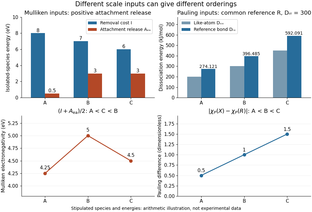
Stipulated inputs to Mulliken electronegativity and arithmetic-baseline Pauling electronegativity: different energies, units and orderings
. Details. 
Independently stipulate and for , with unlike-atom valuesThus , and the Pauling scale differences from are . If all three fictitious species are placed above on that scale, their ordering is , whereas the stipulated Mulliken scale gives . The bond-dissociation energies and isolated-species energies were invented independently: this demonstrates what the formulas do, not a measured disagreement for actual chemical elements. A unit conversion cannot force these two input models to agree.
Mulliken electronegativity uses both the cost of removing an electron and the energy released by accepting an electron. For specified isolated-atom states, the common ground-state convention isThe free electron's energy is the zero reference. Here is the ionization energy and is the electron affinity, positive for exothermic attachment. If attachment is instead tabulated as the signed energy change , the same expression is . Stating the sign convention prevents adding the wrong quantities. The 1934 original treated suitable valence states, which are not automatically the ground states used in this example.[ref]
Mulliken electronegativity has energy units before any additional rescaling. With and in electronvolts per chemical atom, is in electronvolts; with both in , it is a molar energy. For hydrogen, the RSC ground-state inputs are and , giving per chemical atom. For chlorine, and give . These are calculated ground-state Mulliken electronegativities, not the RSC's tabulated Pauling electronegativities.[ref][ref]
Both schemes place chlorine above hydrogen here, but their numerical differences cannot be subtracted from one another or equated. Dividing a molar Mulliken electronegativity by an energy conversion factor changes units; it does not transform it into a Pauling electronegativity. A further empirical mapping would require its own calibration and stated domain.
Pauling electronegativity is a relative, dimensionless scale motivated by bond-dissociation energies. The interesting observation is that a chemical bond between unlike chemical atoms can be stronger than a simple baseline inferred from the corresponding like-atom chemical bonds. An empirical excess energy can then be associated with an electronegativity difference. The 1932 paper The Nature of the Chemical Bond. IV. The Energy of Single Bonds and the Relative Electronegativity of Atoms built such a map; its original coordinates used hydrogen as zero, so those coordinates should not be mistaken for the modern tabulated Pauling electronegativities.[ref]
One arithmetic-baseline version of the Pauling scale relation isHere , and are consistently defined bond-dissociation energies per molecule, and the arithmetic mean is the chosen baseline. With molar energies instead, write , approximately . The denominator makes the result dimensionless; the factor is not a unit-independent magic constant. This is an empirical relation with a specified baseline, not a definition valid for every chemical bond.[ref]
Energy Electronegativity and Chemical Bonding by Stepan S. Batsanov. §1 equation (1), coefficients for eV, kcal/mol and kJ/mol; §2.2, dependence on other bond properties
For an explicitly synthetic example, suppose and with the same temperature and dissociation convention. Then and the model gives an electronegativity difference of . Replacing by gives zero; a negative excess would make this real square-root model inapplicable, not produce a negative electronegativity difference. These invented inputs illustrate the formula and are not measurements of named chemical substances.
Only differences appear, so adding the same constant to every Pauling electronegativity leaves this relation unchanged. A reference value must fix the origin. The bond-dissociation energies alone also do not tell which endpoint attracts electron density more strongly, because interchanging and leaves the formula unchanged. Chemical comparisons fix that direction. Thus Pauling electronegativity is useful as a compact ordering, while the underlying measured energies and approximations remain essential.
An electron shell collects the allowed electronic quantum states sharing a principal quantum number . Its occupancy is the number of electrons assigned to those states in an electron configuration. An electron shell is not a material surface or a prescribed orbit.
Electromagnetism lecture notes by Richard Fitzpatrick Laws of Geometric Optics by Codex 0 2026-10-13
Codex 0 2026-10-13Cited passages: Richard Fitzpatrick, Laws of Geometric Optics, equations 949–955: tangential wavevector matching and refraction; Richard Fitzpatrick, Laws of Geometric Optics, equations 951–953 and accompanying definition of the vacuum wavenumber.
For a differential one-form on an oriented three-dimensional spacetime, varying , with , gives . With signature , on one- and two-forms; writing gives and the identity . An Abelian gauge transformation changes the action by . Thus the bulk field equation is invariant, while invariance of the integrated action depends on boundary conditions.
Bioelectromagnetism studies electric fields, electric currents and magnetic fields associated with living systems and their interaction with applied fields. Ionic currents across and along biological cell membranes generate measurable signals; the surrounding tissue conducts and redistributes them.
In electrocardiography, surface electrodes measure electric potential differences produced by distributed cardiac activity rather than directly recording one isolated cell. A volume conductor model relates internal source currents to those surface readings. Electrode position and conducting geometry matter, so a changed voltage can reflect source activity, measurement contact or the current paths through tissue.
The electromagnetic field tensor action differs from the component-gradient potential action by . Integration by parts expresses this term as a boundary integral plus . With the Lorenz gauge and fixed or vanishing boundary data, the two actions therefore differ only by a boundary term. Varying the component-gradient action without restriction gives the potential wave equations; the Lorenz condition must be supplied to recover all Maxwell equations.
A thermoelectric effect couples heat transfer and the transport of electric charge: a temperature gradient can generate an electromotive force, while an electric current can carry heat and cause heating or cooling at a junction of different materials. This coupling makes electrical measurement of temperature possible through a thermocouple, and permits conversion of a sustained flow of heat into electrical work. A finite open-circuit voltage does not itself deliver power: electrical power requires an electric current through a load. Thermoelectric conversion therefore involves both electromagnetism and thermodynamics. [ref]
https://thermoelectrics.matsci.northwestern.edu/thermoelectrics/history.html. Northwestern thermoelectrics research group: thermoelectric effects and applications
.A nonelectrolyte supplies neutral molecules rather than ions on dissolving in the specified solvent, as illustrated by sucrose in water.
For example, dissolving an idealized sucrose inventory gives dissolved sucrose molecules, rather than separate cations and anions. Dissolving the same amount of substance of a fully dissociated one-to-one strong electrolyte instead gives of each ion. Both can disappear visibly into the solvent; the resulting chemical species distinguish them.[ref]
A nonelectrolyte is not necessarily insoluble: sucrose provides a soluble counterexample. Nor does the label assert exactly zero measured electrical conductivity. Self-ionization of water, impurities or residual electrolyte from a probe can supply background ions. Comparing with a solvent blank and rinsing between samples, as in the strong electrolyte experiment, tests whether the dissolved substance itself produces appreciable additional mobile ions. This separates visible dissolution from ion production without treating lamp darkness as an absolute absence of electric charge.
A weak electrolyte yields only a fraction of ions from its dissolved substance under the specified conditions, as illustrated by acetic acid in water.
For a neutral weak acid, unconverted molecules coexist with hydronium and the conjugate base at chemical equilibrium. The weak acid dissociation fraction describes the partition of the dissolved inventory; the acid dissociation constant describes the chemical equilibrium at fixed solvent, temperature and standard states. A single fraction is not a permanent label for every concentration: dilution can increase that fraction while the acid dissociation constant stays fixed. Calling a substance a weak electrolyte does not mean its chemical solution must be dilute.[ref]
14.3 Relative Strengths of Acids and Bases. Chemistry 2e, §14.3, Acid and Base Ionization Constants, percent-ionization discussion preceding Example 14.7
The following ideal weak electrolyte dilution law makes the distinction quantitative for a monoprotic acid. Other weak electrolytes, mixed chemical solutions and additional proton-transfer steps require their own chemical equilibrium and inventory balances.
A strong electrolyte yields essentially all ions from its dissolved substance in the specified solvent and conditions. Strength does not specify concentration.
For dissolved sodium chloride in dilute water, one dissolved formula unit supplies one sodium cation and one chloride anion. For hydrogen chloride in water, ions instead arise by proton transfer to the solvent, giving hydronium and chloride. Thus separating existing ions by dissociation of an ionic compound and producing ions from neutral molecules by ionization can both give a strong electrolyte.[ref]
The denominator in “essentially all” is the dissolved inventory. Solubility asks how much enters the chemical solution; electrolyte strength asks what happens to the part that enters. A sparingly soluble ionic compound can therefore have an essentially fully dissociated dissolved portion. Undissolved solid does not count as neutral dissolved chemical species, and low electrical conductivity alone does not establish a weak electrolyte.[ref]
11.2 Electrolytes. Chemistry 2e, §11.2, Ionic Electrolytes, paragraph on sparingly soluble ionic compounds
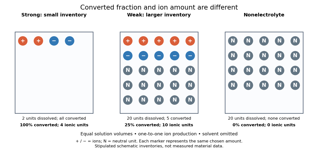
Electrolyte strength and dissolved amount of substance answer different questions
. Original schematic inventories in equal volume of a specified solvent. Each symbol represents the same chosen amount of substance, not one literal microscopic sample. A two-unit strong electrolyte inventory produces two cations and two anions; a twenty-unit weak electrolyte inventory with a stipulated one-quarter converted fraction produces five of each ion and fifteen neutral units. A twenty-unit nonelectrolyte inventory remains neutral. The solvent and its background ions are omitted. These are chosen inventories, not measured material data. Details.
The diagram's weak electrolyte has the smaller converted fraction but more ions in the same volume: ten charged symbols versus four. Even at equal total ion concentrations, different ion drift velocities can give different electrical conductivities. Strength is useful for predicting dissolved chemical species in chemical equations; concentration and transport properties are additionally needed to predict electric current.
An inspected motivating experiment is Harvard Natural Sciences Lecture Demonstrations' Conductivity of Solutions by Harvard Natural Sciences Lecture Demonstrations, Setting it Up. Separate labeled beakers hold aqueous sodium chloride, sucrose, acetic acid and hydrochloric acid samples specified at , with about in beakers; distilled water supplies a blank. Metal electrodes enclosed in tubing connect to a lamp. The readout is lamp brightness; the page reports that an ionic chemical solution lights the lamp. A separate deionized-water rinse station limits carryover between samples.[ref]
Conductivity of Solutions by Harvard Natural Sciences Lecture Demonstrations. Setting it Up, sample list, enclosed electrodes, lamp and rinse station
For a controlled interpretation, keep electrode spacing and immersed area fixed, compare at the same temperature, and recheck the blank after rinsing. These are additional controls: the page supplies no numerical electrode geometry, temperature or calibration. Brightness supports the presence of mobile ions; it cannot alone measure the converted fraction because concentration, ion mobility and circuit response also matter. Its classification of insoluble compounds as weak should not replace the dissolved-inventory distinction above.[ref]
Conductivity of Solutions by Harvard Natural Sciences Lecture Demonstrations. How it Works and Setting it Up; qualitative readout and unspecified geometry and temperature
An electrolytic cell uses an external source of electrical work to drive electrode chemical reactions. In the ordinary two-terminal driven mode, its positive anode supports oxidation and its negative cathode supports reduction. The source removes electrons from the anode and supplies electrons to the cathode; through the electrolyte, net conventional current goes from anode toward cathode. Terminal signs refer to the driven cell's terminals relative to each other. The source supplies electrical power to the cell. See 17.7 Electrolysis (§17.7: electrolysis and electroplating).
For example, transferring copper from a soluble copper anode onto a conducting object at the cathode has the ideal half-reactionsTheir sum transfers copper between surfaces. For identical bulk states, this transfer need not have a positive bulk Gibbs free energy change; finite electric current still needs applied drive to overcome losses. Thus "consumes electrical work" does not mean every electrolytic cell stores all that work as chemical Gibbs free energy. Electrolysis can instead redistribute material. The charge-to-amount relation remains when only these half-reactions carry the electric current; competing water reactions would change the deposited amount. The electroplating principle and charge accounting are described in 17.7 Electrolysis (§17.7: electroplating and quantitative aspects).
The University of Washington's teaching demonstration makes this material transfer visible with a copper electrode and a stainless-steel electrode in a glass cell containing . The external source connects its positive lead to copper and negative lead to steel; the reported observation is a copper coating on the steel. Reversing the source polarity removes the deposited copper again: the coated surface now supports oxidation and acts as the anode. This polarity reversal changes the drive, unlike swapping the measurement leads in the Daniell cell voltage and load experiment. Coating appearance alone does not measure charge efficiency or exclude competing chemical reactions. See University of Washington, Electroplating Copper on Stainless Steel: apparatus and reversible coating demonstration.
The copper cathode in this driven example is negative, while the copper cathode of a discharging Daniell cell is positive: both support exactly the same reduction half-reaction. Likewise, an anode need not lose material if its conducting surface is absent from its net half-reaction. Neither terminal sign nor a universal mass-change rule defines an anode or cathode.
There are unlisted articles, also show them or only show them.