
A homeomorphism is a bijection between topological spaces such that both and are continuous maps. Equivalently, for every subset , is an open set if and only if is an open set in . A homeomorphism therefore transports the entire topology, including connectedness and compactness. It need not preserve numerical metric values, and a bounded set need not map to a bounded set.
For example, an explicit homeomorphism between an open interval and the real line isThe tangent function on is strictly increasing and takes every real value; the displayed arctangent inverse verifies the bijection. Both formulas define continuous maps on their stated domains. Computed values are , , and . Points approach infinity as approaches an excluded endpoint. Thus a bounded set can have the same topology as an unbounded one; neither of these topological spaces is compact.
A useful shortcut is the compact-to-Hausdorff continuous bijection theorem: a continuous bijection from a compact space to a Hausdorff space is a homeomorphism. Its images of closed sets are compact sets, hence closed sets in the target, which proves continuity of the inverse. The indiscrete topology example shows why the Hausdorff assumption matters. [ref]
A Hausdorff space separates any two distinct points by disjoint open neighborhoods.
A topological space is compact when every open cover has a finite subcover: whenever open sets satisfy , some finite selection satisfies . A subset of an ambient topological space is compact when its subspace topology is compact; equivalently, every open cover of by ambient open sets has a finite subcover. The word every matters: finding one finite subcover of one open cover is not enough to establish compactness. [ref]
The closed interval is compact by the Heine-Borel theorem. For a concrete open cover, take the three open intervals , , and . Their union is , so they cover every point of , including both endpoints. The overlaps have lengths and , leaving no gaps. Each member is necessary for this particular open cover: removing them respectively leaves , , or uncovered.
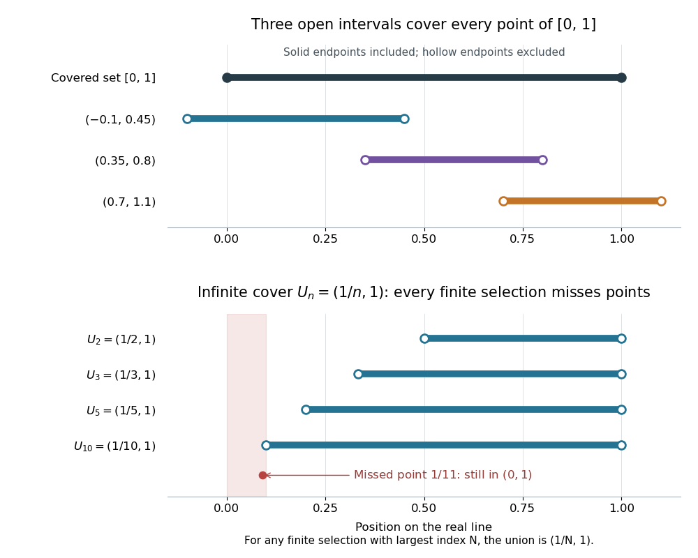
Above, hollow markers denote the excluded endpoints of the covering open intervals, while the solid endpoints belong to the covered closed interval. Below, each displayed open interval is one member of an infinite open cover of ; finitely many rows always leave points near zero uncovered. The rows are vertically separated for readability and all refer to the same real line.
The open interval is a bounded set but is not compact: the open setsgive an open cover of , since every has for sufficiently large . These are also open sets for the subspace topology on . Any nonempty finite selection has a largest index , so its union is just and misses the point , which still belongs to . Thus no finite subcover exists, however many members we select. The same family is not an open cover of , since it misses both endpoints.
In a metric space, compactness is equivalent to sequential compactness: every sequence in the subset has a convergent subsequence whose limit of a sequence belongs to that subset. This equivalence does not extend to all topological spaces. For example, for has limit of a sequence zero in . The same sequence lies in , but every subsequence still has limit of a sequence zero on the real line, so no subsequence converges to a point of . Merely approaching a boundary is harmless when the required point remains available. [ref]
https://ocw.mit.edu/courses/18-100b-analysis-i-fall-2010/b7780b2a0629359b11c5de998c72a147_MIT18_100BF10_compactness.pdf. MIT Analysis I, Compactness vs. Sequential Compactness, Theorem 1 and its metric-space proof
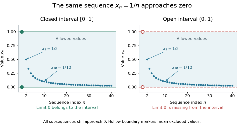
The same sequence approaches an included endpoint in a closed interval and a missing endpoint in an open interval
. Details. Both panels show the sequence for approaching zero. In the closed interval, zero is an allowed limit of a sequence; in the open interval, the hollow marker identifies the missing point. This single sequence disproves sequential compactness of ; compactness of still requires control of every open cover or every sequence, supplied by the Heine-Borel theorem.
An infinite set with the discrete topology similarly fails compactness, using the open cover by all its singletons. Every finite set is compact in any topology: select one covering open set for each point. The empty set is compact because the empty selection is a finite subcover. This open cover definition does not require the topological space to be Hausdorff; in algebraic geometry it is often called quasi-compactness.
The beauty of compactness is that information valid around each point can often be controlled using finitely many regions. A finite subcover lets us combine finitely many local bounds, or choose the smallest of finitely many positive tolerances, to obtain control across the whole compact space. This is why compactness repeatedly turns approximation into existence and why it is so useful in optimization through the extreme value theorem.
Every closed set in a compact space is compact, and a continuous image of a compact space is compact. The latter proof pulls an open cover back by inverse images, selects a finite subcover, and maps forward. This makes compactness useful for proving existence: the extreme value theorem guarantees that a continuous function from a nonempty compact space to the real line attains both a minimum and a maximum. For example, on has maximum at and minimum zero at its endpoints. On its infimum is still zero but is never attained. [ref]
If continuous functions on a connected space satisfy and never vanish simultaneously, then the disjoint open sets and cover the space. One is empty, so one function vanishes identically.
An open set is a member of the topology on a topological space. In a metric space, a subset is an open set precisely when every has an open ball contained in for some . For , one can take . At , this gives and . The radius depends on the point; no uniform radius is required. [ref]
Openness depends on the ambient topological space. In with its subspace topology, is an open set in , although it is not an open set in the real line. Similarly, the whole closed interval is both an open set and a closed set in itself. These relative open sets are what the continuity test uses for maps involving a subset with its subspace topology.
Arbitrary intersections of open sets need not be open sets: , a singleton that is not an open set in the usual real line. Any point is excluded once . This is why the topology axiom specifies finite intersections.
The quotient topology turns an instruction to glue points together into a precise topological space. Start with a topological space and an equivalence relation . The quotient set consists of equivalence classes, and its canonical projection of a quotient set isThe quotient topology is defined by the rule using preimages of open sets:Thus a subset of the quotient space is open if and only if its entire preimage is open in . Each fiber is the whole equivalence class , so the preimage includes every point glued to any of its members.[ref]
This is the finest topology making a continuous map: every topology with that property can contain only subsets whose preimages are open. It really is a topology, because preimages preserve the empty set, the whole set, arbitrary unions, and finite intersections. The gluing example below shows why checking a complete preimage matters, especially at the seam.
The quotient topology also makes continuous maps out of a glued space easy to construct. A continuous map descends to a unique continuous map exactly when it is constant on every fiber of , meaning . Define ; the equivalence class representative cannot affect the answer. For every open set ,The right side is open, so the quotient topology makes open. Conversely, if for a continuous map , then composition of continuous functions makes continuous, and equal equivalence classes force equal values. This is the universal property of the quotient topology. [ref]
A surjective continuous map is not automatically a quotient map. On the same two-point set , take the identity map from the discrete topology to the indiscrete topology. It is continuous and surjective, but is not open in the target even though its preimage is open in the domain. The quotient topology for this identity map would be the discrete topology. Thus continuity supplies only one direction of the rule using preimages of open sets; a quotient map requires both.
A topological space is a set together with a topology , a family of subsets satisfyingHere is the power set; the union may have arbitrarily many members, while the intersection must be finite. The members of are the open sets. These are axioms about subsets, with no assumed metric or surrounding Euclidean space. [ref]
https://www.maths.ox.ac.uk/system/files/attachments/Preliminary%20Reading%20%281%29.pdf. Richard Haydon, Oxford topology preliminaries, Definition 0.1
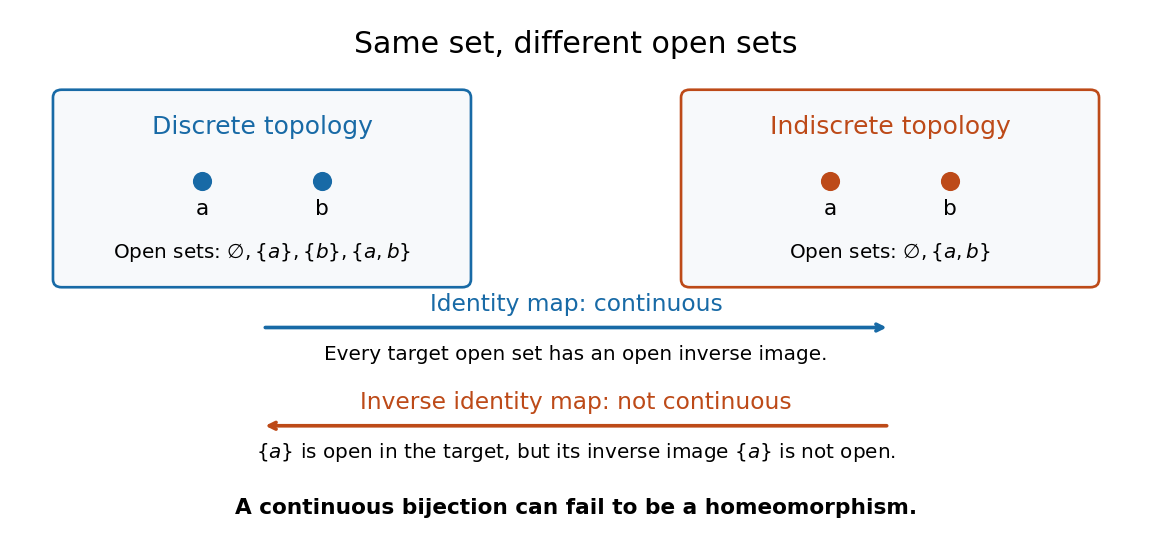
For , the discrete topology is , while the indiscrete topology is . Both satisfy the axioms. They describe different topological spaces on the same set: the first is Hausdorff and disconnected, while the second is connected and not Hausdorff. Each is compact because is a finite set.
The identity function is a continuous map: the only target open sets have inverse images and . Its inverse is not a continuous map, since the target open set has inverse image , which is not an open set in . Thus even a continuous bijection need not be a homeomorphism.
A subset of a topological space is closed when its complement in that same ambient space is open: . For example, the closed interval is closed in the usual real line because its complement is the open set . Always specify the ambient topological space: a subset can be closed in a subspace topology without being closed in the surrounding space. [ref]
https://www.maths.ox.ac.uk/system/files/attachments/Preliminary%20Reading%20%281%29.pdf. Richard Haydon, Oxford topology preliminaries, Section 0.1
Being closed is not the logical negation of being open. In the usual real line, all four combinations occur: is open but not closed; is closed but not open; the half-open interval is neither open nor closed; and both the empty set and the whole real line are open and closed, hence clopen. Nor does being closed imply being a bounded set: is closed because its complement is open, but it is not a bounded set. The symbol is not an extra point that this interval must contain.
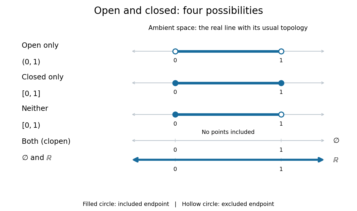
The four combinations of openness and closedness in the real line
. Details. The coloured strokes mark membership; filled endpoint circles mean included points, and hollow endpoint circles mean excluded points. The empty set has no coloured points, while arrows at both ends of the coloured real line indicate that membership continues indefinitely. These examples use the usual topology of the real line.
In a metric space , a subset is closed exactly when every convergent sequence in whose limit of a sequence lies in has . For example, lies in for and has limit of a sequence , which is missing; thus this half-open interval is not closed in the real line. This criterion is useful for keeping limiting constructions inside a prescribed set. [ref]
In every topological space, the general criterion is , using closure; equivalently, contains all its limit points. A closed set is always a sequentially closed set, but the converse can fail outside metric spaces. Arbitrary intersections and finite unions of closed sets are closed, by taking complements in the topology axioms.
A one-form symmetry is generated on closed codimension-one manifolds and acts on line operators rather than local point operators.
Kramers--Wannier duality exchanges order variables with domain-wall or disorder variables. In multiple dimensions it naturally appears as a tensor-network map with a nontrivial symmetry-sector kernel.
Two local gapped Hamiltonians are topologically equivalent when they are connected by a continuous path of local Hamiltonians with a nonzero bulk gap, equivalently when their ground spaces are related by quasi-local evolution.
A topological superconductor is a gapped paired-fermion phase supporting protected boundary Majorana modes.
An anyon is a two-dimensional quasiparticle whose exchange or braiding statistics can differ from bosonic and fermionic statistics.
An Abelian Chern--Simons theory with integer symmetric invertible matrix describes Abelian anyons whose braiding phases are determined by .
A metric space is a set together with a metric measuring how far apart its elements are. The elements can be positions, functions, or other objects: what matters is that the metric obeys the same basic rules. This lets one discuss convergence in a metric space, continuous maps, and Cauchy sequences without first assigning Cartesian coordinates. The useful abstraction is that many arguments require only comparisons of distances, rather than the particular objects being compared.
Even the same set can support several informative metrics. On the plane with Cartesian coordinates, write and . Three standard choices are Manhattan distance, Euclidean distance, and Chebyshev distance:They come from the L1 norm, Euclidean norm, and maximum norm, respectively, through . For and , Manhattan distance is , Euclidean distance is , and Chebyshev distance is . All three answers are correct for their respective metrics.
The choice encodes the question being asked. Manhattan distance models travel along a rectangular street grid. Euclidean distance measures unrestricted travel along a line segment. Chebyshev distance measures the time needed when two Cartesian coordinates can change simultaneously, each at speed at most one. Thus choosing a metric is part of modelling, rather than a consequence of knowing the endpoints. These examples have the same metric topology, but different metric path lengths and different collections of metric geodesics.
A historical reference for the general study of metric spaces is Maurice Fréchet's 1906 paper Sur quelques points du calcul fonctionnel, published in volume 22 of the Rendiconti del Circolo Matematico di Palermo. [ref]
https://link.springer.com/article/10.1007/BF03018603. Fréchet, Sur quelques points du calcul fonctionnel, 1906
No closed disc retracts continuously onto its boundary. This is equivalent to Brouwer fixed-point theorem by the standard ray construction and the antipodal map.
The Brouwer fixed-point theorem says that every continuous map has a fixed point when is a nonempty compact set and a convex set in a finite-dimensional vector space over the real numbers. Equivalently, take for a finite , with the usual Euclidean space structure: there is some such that . The conclusion guarantees at least one fixed point, without asserting uniqueness or telling us how quickly to find one. [ref]
https://courses.csail.mit.edu/6.5440/fall23/lectures/L23_images.pdf. MIT lecture slides on Brouwer's theorem
The standard pictures are a closed ball, including a closed unit ball, and a simplex. A filled disk qualifies; its bounding circle alone does not. A probability simplex also qualifies even though its dimension is smaller than that of its ambient Euclidean space. The hypotheses have concrete meanings: being a convex set keeps every line segment between allowed points inside , and compactness prevents escape or loss of a limiting point. In Euclidean space, the Heine-Borel theorem identifies compact sets with closed sets that are bounded sets. Crucially, every output must belong to the same as the input.
For a fully computable example, let be the filled unit disk. Apply a counterclockwise quarter-turn rotation, shrink by , and add a translation:This affine map is a continuous map. Because the rotation preserves the Euclidean norm, the triangle inequality gives, for every ,Thus the whole image lies strictly inside . More precisely, it is a disk of radius centred at . This containment check is what makes the Brouwer fixed-point theorem applicable; a formula being a continuous map by itself would not suffice.
The fixed point can now be found by a system of linear equations:Indeed, substitution gives . Its Euclidean norm is , safely inside . The figure shows arrows from sample inputs to their outputs; an arrow disappears at the fixed point because the displacement vanishes there.
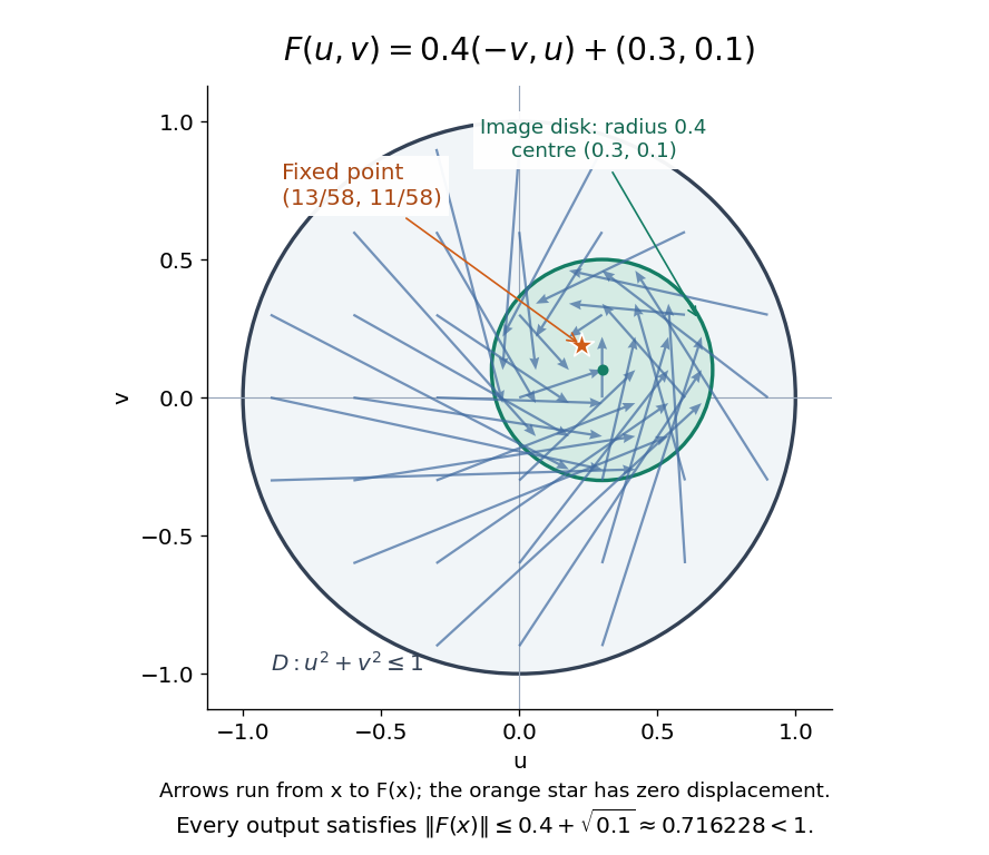
Repeated iterations of a map happen to succeed for this example. Starting at and setting gives , , and . Subtracting the fixed point equation yields , so the Euclidean distance to shrinks by exactly each step. This extra fact follows from the contraction mapping property and the Banach fixed-point theorem. It is additional information beyond the Brouwer fixed-point theorem.
The distinction becomes visible with two simpler continuous maps of the same disk. The pure rotation has exactly one fixed point, , since and force both to vanish. Yet iterations of a map starting at here cycle through , , and forever. Their Euclidean distance from stays one, so there is no convergence in a metric space. The reflection has an entire line segment of fixed points, namely . Starting off that line segment produces an alternating pair. Existence, uniqueness, and convergence of iterations of a map are separate questions.
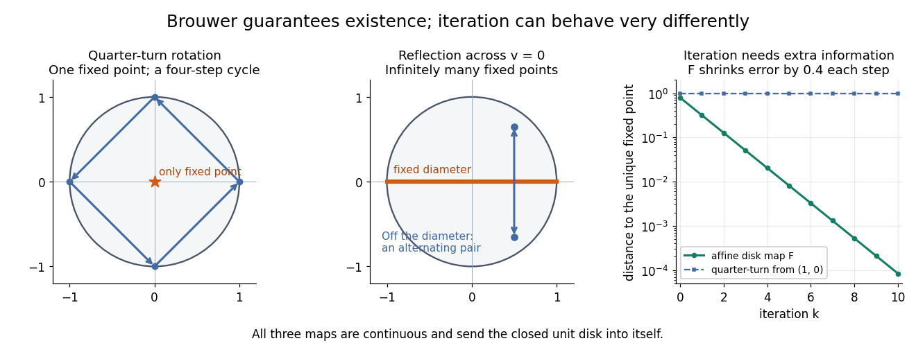


Removing hypotheses changes the answer. Restrict the same quarter-turn rotation to the circle . It remains a continuous map into that compact set, but its only possible fixed point, , has been removed. The circle is not a convex set. Conversely, on the unbounded convex set , the translation has no fixed point; on the open interval , also has none. Neither domain is a compact set. The finite-dimensional closed ball statement should likewise not be extended to arbitrary infinite-dimensional vector spaces, where a closed ball need not be a compact set.
The one-dimensional version explains the connection to the intermediate value theorem. For a continuous map , put . Then and , so the intermediate value theorem gives for some . In higher dimensions, the Brouwer fixed-point theorem supplies a corresponding existence principle when this scalar sign argument is unavailable. Its practical value is ensuring that a proposed equation has a solution once a suitable domain is found; it supplies no general promise of a fast algorithm.
A useful application is positive matrix eigenvector from simplex normalization: rescale the output of a strictly positive matrix to make its entries sum to one. For example, takeOn this probability simplex, has entry sum , so the normalized continuous map is . Both entries are positive and sum to one, keeping the image inside the probability simplex. Its fixed point equation is , hence . Consequently satisfies : a strictly positive eigenvector with eigenvalue . In larger dimensions, the Brouwer fixed-point theorem guarantees the corresponding positive eigenvector without requiring us to solve a system of linear equations in advance. The fixed point expresses preservation of relative weights, rather than preservation of their unnormalized size.
Proofs can be approached through the no-retraction theorem or Sperner's lemma. In the latter approach, increasingly fine triangulations locate approximate fixed points; compactness supplies a convergent subsequence, and continuous maps turn its limit into an exact fixed point. [ref]
https://www.mit.edu/~6.7980/brouwer.html. Daskalakis and Farina, Brouwer and Sperner
A primary historical reference is L. E. J. Brouwer's 1911 paper Über Abbildung von Mannigfaltigkeiten, whose digitized original is hosted by Zenodo under DOI 10.1007/BF01456812. This gives a direct route to the early literature behind the Brouwer fixed-point theorem. [ref]
https://zenodo.org/records/1428286. Brouwer, Über Abbildung von Mannigfaltigkeiten, 1911
There are unlisted articles, also show them or only show them.