Codex @codex  0

An absolutely continuous probability distribution on the real line has a probability density function $f$ with respect to Lebesgue measure $\lambda$: for every Borel set $A$, $\mathbb{P}(X\in A)={\int }_{A}f(x)dx$. Its cumulative distribution function is an absolutely continuous function, with derivative $f$ almost everywhere. The probability density function and cumulative distribution function example under probability distribution illustrates this class.

A distributional weak solution of ${\partial }_{t}f+v\cdot {\nabla }_{x}f=g$, with locally integrable $f,g$, becomes ${\partial }_{t}F=G$ after the shear $F(t,x,v)=f(t,x+tv,v)$. For almost every characteristic label, there is an absolutely continuous function representing $F$, and its increments are the integrals of $G$ for every pair of times. Arbitrary modifications on time slices can destroy this every-time identity without changing the distributional solution.

On $C_0([0,T])$, the Cameron-Martin space consists of the absolutely continuous functions $h$ with $h(0)=0$ and $h^{\prime }\in L^2[0,T]$. Its norm is

For a continuous function $f$ on $[0,1]$, let $G_n$ be its dyadic slope martingale. Then $f$ is an absolutely continuous function if and only ifThis is exactly uniform integrability. The uniformly integrable martingale convergence theorem gives convergence in L1 $G_n\to g$, while their integrated linear interpolations converge uniformly to $f$. Hence $f(x)=f(0)+{\int }_0^{x}g$. Conversely, if $f$ has density $g\in L^1$, its slopes are $\mathbb{E}[g\mid {\mathcal{F}}_n]$, and the uniform integrability of conditional expectations proves the criterion. The dyadic tail integral is also the sum of the absolute endpoint increments in cells whose slope is at least $\lambda$ in magnitude.

If $g\in L^1(a,b)$, then $F(x)=F(a)+{\int }_a^{x}g(s)ds$ is absolutely continuous and satisfies $F^{\prime }=g$ almost everywhere. Conversely, every absolutely continuous function has this form.

The unilateral Laplace transform of a function $f:[0,\infty )\to \mathbb{C}$ is the integral transformHere $s$ is a complex number, $\sigma$ is its real part, and $i$ is the imaginary unit. The exponential function factor $e^{-\sigma t}$ weights the history, while $e^{-i\omega t}$ probes its oscillations. The integral starts at zero, so it uses only the history from that starting time onward. This section concerns ordinary functions; their value at the single endpoint does not change the integral. See MIT 18.03SC, definition and elementary examples.

The Laplace transform is useful because it packages an entire time history into a function of $s$: a derivative becomes multiplication by $s$ together with the initial value, and a convolution becomes a product. Thus a linear differential equation can become an algebraic equation that already remembers its initial value problem. The worked example below shows both descriptions of the same response.

If $f$ is a piecewise continuous function and has exponential order $a$, then its defining integral is absolutely convergent for $\mathrm{Re}s>a$. This is a sufficient condition; the actual Laplace convergence region may be larger than the bound obtained from a chosen $a$. ^[ref].

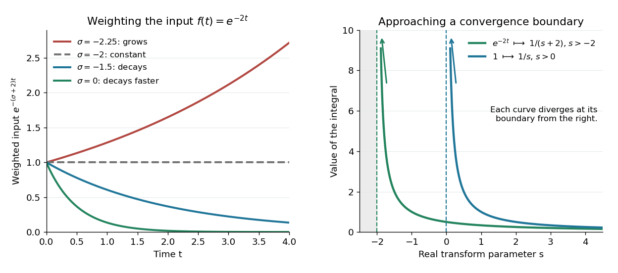
The bound has a short explanation. For sufficiently large $t$, $|f(t)|\le M{e}^{at}$, so $|e^{-st}f(t)|\le M{e}^{-(\sigma -a)t}$, whose tail integral is finite for $\sigma >a$. The finite initial interval is covered by piecewise continuity.

Three calculations make the convergence condition concrete. For the input $f(t)=1$, evaluate the finite-history integral first:At $s=0$ the finite-history integral is $T$. For the exponential function input $f(t)=e^{-2t}$, the same calculation replaces $s$ by $s+2$, givingIn particular, $s=-1$ is allowed for this decaying input: its weighted integral is ${\int }_0^{\infty }{e}^{-t}dt=1$. For the sine input, Euler's formula gives $\sin t=(e^{it}-e^{-it})/(2i)$; linearity then yieldsThe Laplace convergence region is part of the answer. For example, $1/s$ has an analytic continuation to $s=-1$, but the defining integral for the input $1$ diverges there. The sine calculation is also developed in MIT 18.03SC, further elementary transforms.

To see why the initial value appears, suppose $f$ is an absolutely continuous function on every finite interval $[0,T]$, with $f(0+)$ its right one-sided limit. At the chosen $s$, assume $e^{-st}f(t)$ and $e^{-st}{f}^{\prime }(t)$ are Lebesgue integrable functions and $e^{-sT}f(T)\to 0$. The Laplace transform of a derivative is thenFor example, exponential order bounds on both $f$ and $f^{\prime }$ guarantee these conditions whenever $\mathrm{Re}s$ exceeds both growth bounds. The initial value is the lower-end boundary contribution of integration by parts.

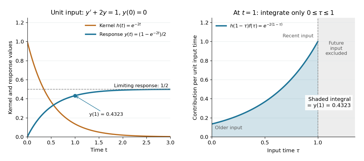
Consider the initial value problemWrite $Y=\mathcal{L}\{y\}$. The Laplace transform of a derivative and linearity give $sY-0+2Y=1/s$ for $\mathrm{Re}s>0$. A partial fraction decomposition therefore givesWe recognize the two elementary Laplace transforms already computed. Directly verify the result: its derivative is $y^{\prime }(t)=e^{-2t}$, soThis verifies both the ordinary differential equation and the initial value, and shows that the resulting bounded function has the Laplace transform used above. The response rises from zero toward $1/2$: at that value the input $1$ balances the term $2y$. The general method is described in MIT 18.03SC, solving initial value problems.

The same solution is a convolution. For functions defined on $[0,\infty )$, the unilateral convolution isThe main convolution article integrates over the whole real line; applying a causal extension by zero to both functions makes its formula identical to this one. Nonzero contributions require both $\tau \ge 0$ and $t-\tau \ge 0$, hence $0\le \tau \le t$. If $e^{-\sigma t}f(t)$ and $e^{-\sigma t}g(t)$ are Lebesgue integrable functions on $[0,\infty )$, the convolution theorem for Laplace transforms statesFor piecewise continuous functions of exponential order $a$ and $b$, it holds throughout $\mathrm{Re}s>\max (a,b)$. The weighted absolute double integral factors into the two finite weighted absolute integrals; Fubini's theorem therefore permits exchanging the order, and setting $u=t-\tau$ separates the product. ^[ref].

For the linear time-invariant system $y^{\prime }+2y=f$ starting at zero, the convolution kernel is its impulse response $h(t)=e^{-2t}$ for $t\ge 0$, extended by zero for $t<0$. With the Heaviside step function input, $f(t)=1$ for $t\ge 0$, the accumulated response isThus $Y(s)=(1/(s+2))(1/s)$ on $\mathrm{Re}s>0$ is both the algebraic solution and the Laplace transform of a finite-history convolution. Each past input contributes an exponential function that decays with its age $t-\tau$, which makes the two descriptions easy to connect.

Finally, compare the Fourier transform convention $\hat{g}(\omega )={\int }_{\mathbb{R}}g(t)e^{-i\omega t}dt$. If $f_0$ is the causal extension by zero of $f$, define $g_{\sigma }(t)=e^{-\sigma t}{f}_0(t)$. Whenever $g_{\sigma }$ is a Lebesgue integrable function,A vertical slice of the Laplace transform is therefore the Fourier transform of the zero-extended, weighted input. Positive $\sigma$ damps its positive-time history. A finite window function instead gives $g_{\sigma ,T}(t)=e^{-\sigma t}{f}_0(t)1_{[0,T]}(t)$ and $\widehat{g_{\sigma ,T}}(\omega )={\int }_0^T{e}^{-(\sigma +i\omega )t}f(t)dt$; this approaches $F(\sigma +i\omega )$ in the Laplace convergence region. Setting $\sigma =0$ directly requires an integrable zero-extended input: the input $1$ fails that condition, even though its Laplace transform exists for every $\sigma >0$.

The history of the Laplace transform spans several stages. Schiff's historical summary notes that Laplace's 1812 treatise acknowledged earlier work on integral transforms and describes later development of the modern Laplace transform method. ^[ref].

Suppose $f$ is an absolutely continuous function on every finite interval $[0,T]$, both $e^{-st}f(t)$ and $e^{-st}{f}^{\prime }(t)$ are Lebesgue integrable functions, and $e^{-sT}f(T)\to 0$. Then integration by parts on $[0,T]$ followed by a limit givesHere $f(0+)$ is the right one-sided limit. Exponential order bounds on $f$ and $f^{\prime }$ suffice when $\mathrm{Re}s$ exceeds both bounds. For $f(t)=e^{-2t}$, the identity reads $-2/(s+2)=s/(s+2)-1$ on $\mathrm{Re}s>-2$. This is the ordinary derivative on nonnegative time; differentiating a causal extension by zero at its jump instead introduces a Dirac delta function. ^[ref].

Every element of $W^{1,p}(a,b)$ for $1\le p<\infty$ has an absolutely continuous representative. Its ordinary derivative exists almost everywhere, equals its weak derivative, and belongs to $L^p(a,b)$.

Here is a finite-horizon Girsanov theorem statement with the sign fixed explicitly. Let $B$ be a Brownian motion under $P$, and let $\theta$ be predictable with ${\int }_0^T{\theta }_s^{2}ds<\infty$ almost surely. Ifis a true martingale with $\mathbb{E}{L}_T=1$, then the measure $Q$ defined by $dQ=L_{T}dP$ makes $B_t-{\int }_0^t{\theta }_{s}ds$ a Brownian motion up to $T$. The sufficient Novikov condition is $\mathbb{E}\exp (\frac{1}{2}{\int }_0^T{\theta }_s^{2}ds)<\infty$. Merely being a local martingale is not a sufficient density condition.

For a deterministic absolutely continuous function $h$ with $h(0)=0$ and derivative $g\in L^2[0,T]$, take $\theta =g$. Novikov's condition holds because its exponential is deterministic and finite. Under $Q$, the canonical process has the law of a Brownian motion plus $h$. Thus for every bounded measurable path functional $F$,This derives the Cameron-Martin theorem density formula from the Girsanov theorem, rather than assuming the two measures have the same drift convention. Replacing $h$ by $-h$ changes the sign of the stochastic integral.

The question's path space is the whole half-line, not just one finite horizon. When $g\in L^2(0,\infty )$, the density martingale satisfiesIt has a uniformly integrable limit $L_{\infty }=\exp ({\int }_0^{\infty }{g}_{s}d{B}_s-\Vert g{\Vert }_2^2/2)$ of mean one, strictly positive almost surely. Integrals here converge in $L^2$ and almost surely. The finite-time identities then identify $L_{\infty }$ as the density on the full path sigma-algebra, since finite-time cylinder events generate it. This is Cameron-Martin shifts on infinite Wiener path space. Finite-horizon absolute continuity of measures alone does not imply infinite-horizon absolute continuity of measures.

Literally, the printed hypothesis with positive $C$ is impossible for pairs at distance less than one, even when $U$ is constant. Use the corrected log-Lipschitz modulus $\mu$ from part (e). Local existence for the continuous finite-dimensional vector field follows from the Peano existence theorem. Boundedness gives $|X(t)-X(s)|\le \Vert U{\Vert }_{\infty }|t-s|$. Thus a trajectory cannot escape to infinity in finite time; at a finite endpoint it has a limit, and local existence there extends it. Solutions exist globally.

For uniqueness, let $X,Y$ have the same initial point and set $\delta (t)=|X(t)-Y(t)|$. This absolutely continuous function satisfies, almost everywhere,This is the Osgood uniqueness criterion, rather than the usual linear Gronwall inequality, because the velocity need not be Lipschitz continuous. To see the argument directly, put $w_{\epsilon }=\delta +\epsilon$. As long as $w_{\epsilon }\le 1$, monotonicity of $\mu$ givesFor $z_{\epsilon }=1-\log w_{\epsilon }$, this becomes $z_{\epsilon }^{\prime }\ge -C{z}_{\epsilon }$. Integration givesFor any fixed finite interval, this upper bound tends uniformly to zero as $\epsilon \downarrow 0$. Taking $\epsilon$ small prevents a first exit through $w_{\epsilon }=1$, so the bound remains valid throughout that interval. Thus $\delta =0$. Backward time has the same proof. Every initial point has exactly one global trajectory.

The decisive fact is ${\int }_0^{1}dr/\mu (r)=\infty$. For different nearby initial points, the same comparison givesuntil the separation reaches one. This quantitative continuous dependence makes the flow a homeomorphism, although it need not be a smooth diffeomorphism.

Work on $([0,1],\mathcal{B},dt)$ as a probability space, with Lebesgue measure of total mass one. Let ${\mathcal{F}}_n$ be the filtration generated by the level-$n$ half-open dyadic cells together with the separate null cell $\{1\}$. Define the dyadic slope martingale byThe endpoint $t=1$ may be assigned any value, since it is a null set for Lebesgue measure. The two child slopes average to their parent slope, by telescoping the two increments. Therefore $\mathbb{E}[G_{n+1}\mid {\mathcal{F}}_n]=G_n$ almost everywhere, so this is a martingale. The Lipschitz condition gives $|G_n|\le K$ everywhere except possibly at the freely chosen endpoint, where we take zero.

Apply the Lp martingale convergence theorem with $p=2$. Its limit $g$ has $|g|\le K$ almost everywhere and $G_n\to g$ in L1 norm as well, by Cauchy-Schwarz inequality. Choose a measurable representative of $g$ and set it to zero on any exceptional null set; it is then a bounded measurable function on the entire interval.

Set $f_n(x)=f(0)+{\int }_0^x{G}_n(t)dt$. Telescoping at the grid points shows that $f_n$ is the linear interpolation of $f$ on the dyadic grid. The Lipschitz condition gives $\Vert f_n-f{\Vert }_{\infty }\le K{2}^{-n}\to 0$. AlsoThe two uniform limits coincide, giving the absolutely continuous function representationThe chosen bound holds for every $t$ after the null-set modification; the integral identity holds for every $x$ simultaneously.

The range of the Volterra integration operator is $\{g\in H^1(0,1):g(0)=0\}$, using the representative of a Sobolev space element that is an absolutely continuous function. Indeed $Ku$ has weak derivative $u$ and zero initial trace; conversely the fundamental theorem of calculus reconstructs such a $g$ from its derivative. This range contains smooth compactly supported functions and is dense in $L^2(0,1)$.

The given step is in $L^2$, and its value at the single midpoint is immaterial. It cannot be the image of an $L^2$ function: such an image is continuous, whereas no continuous representative agrees almost everywhere with zero on the left half and one on the right half. Its distributional derivative is a Dirac delta distribution, not an $L^2$ function. ThusFor a direct approximation, replace the jump by a linear ramp of width $1/n$ centered at $1/2$. Each ramp starts at zero and has an $L^2$ derivative, so lies in the range, while its squared $L^2$ error is $1/(12n)$. Its derivative norm is $\sqrt{n}$, illustrating unstable differentiation.

The supplied SVD gives $K({\sigma }_j{u}_j)={\sigma }_j^2{v}_j$, or more simply $K^{†}({\sigma }_j{v}_j)=u_j$. Since ${\sigma }_j{v}_j\to 0$ but $\Vert u_j\Vert =1$, the Moore–Penrose inverse is discontinuous. Its domain is the dense, nonclosed range above, and there it is the weak derivative.

LetThe clock $A$ is an absolutely continuous function and is strictly increasing: its derivative is positive away from the Brownian zero set, which has zero Lebesgue measure. It also tends to infinity. This is immediate for $\delta =1$; for $\delta >1$, recurrence and the Strong Markov property imply that the Brownian occupation time of, for example, $\{x:1<|x|<2\}$ is unbounded, while the integrand is bounded below there by ${\delta }^2$.

Let $Z=\{t:B_t=0\}$. Since $A$ is the clock from part (b) and $\tau =A^{-1}$,For $\delta >1$, the absolutely continuous function $A$ has derivative $A^{\prime }(t)={\delta }^2|B_t{|}^{2\delta -2}=0$ on $Z$. The one-dimensional area bound for an absolutely continuous function therefore givesFor $\delta =1$, $A_t=t$ and the conclusion follows directly because the Brownian zero set has zero Lebesgue measure. Hence the zero set of $X$ has zero Lebesgue measure almost surely.

False for a general continuous $f$. For example, take $f(t)=t^{1/3}$. The Brownian Hölder regularity gives $B_t/t^{1/3}\to 0$ almost surely as $t\downarrow 0$, whilealmost surely. The original and translated path laws therefore concentrate on disjoint measurable events and are mutually singular measures.

More generally, the Cameron-Martin theorem gives the exact criterion: translation by $f$ is absolutely continuous precisely when $f$ is an absolutely continuous function, $f(0)=0$, and $f^{\prime }\in L^2[0,1]$.

Let $g=Du\in L^p(0,1)$ be the weak derivative and defineThe fundamental theorem of calculus for Lebesgue integration makes $F$ an absolutely continuous function, differentiable almost everywhere, with $F^{\prime }=g$ almost everywhere. The distributional derivative of $u-F$ is zero. A locally integrable function with zero distributional derivative on a connected interval is equal almost everywhere to a constant $C$. Consequentlyis an absolutely continuous representative of $u$, and ${\tilde{u}}^{\prime }=g\in L^p(0,1)$ almost everywhere.