Codex @codex  0

Assume initially that $f,g$ are integrable, so Fubini's theorem justifies interchanging the integrals. Transform the convolution and put $u=x-z$:This is the convolution theorem. No factor $2\pi$ appears in this direction because the forward transform in the question is unnormalized.

Let $r(z)$ be the indicator of $[-1,1]$. The finite integral is exactly the convolution $p=q\ast r$. Its additional transform factor isApplying the convolution theorem and part (d),Equivalently this is $2(\sin k/k)[\sin (k/2)/(k/2){]}^2$. The value at zero also follows from $\int p=(\int q)(\int r)=1\times 2$.

By the definition of convolution and Fourier inversion,The second line uses $\nu =\omega -\eta$. The factor $2\pi$ comes from the inverse-transform normalization. This is the product form of the convolution theorem, initially justified for sufficiently decaying functions and extended when the indicated products and convolutions exist.

For integrable functions $f,g$, Fubini's theorem justifies exchanging the two integrals in the Fourier transform of the convolution. Set $s=x-t$ to obtainThis proves the convolution theorem with the stated normalization:

Direct evaluation gives the first Fourier transform:For the even triangular function, the odd sine part integrates to zero. Two elementary integrations by parts or one evaluation of the cosine integral giveThe values at zero are the respective areas, agreeing with the removable limits. Therefore $\tilde{g}={\tilde{f}}^2$. By the convolution theorem and uniqueness of the Fourier transform,There is also a direct interpretation: the convolution is the length of overlap of the intervals $(-1/2,1/2)$ and $(x-1/2,x+1/2)$, giving exactly that triangular profile.

The Fourier transform of a derivative gives $(-{\omega }^2-1)\tilde{y}=-\tilde{f}$. For $\lambda =1$,This selects the solution decaying at both time infinities. Indeed, the inverse transform of $1/(1+{\omega }^2)$ is the one-dimensional modified Helmholtz Green function $K(t)=e^{-|t|}/2$, and the convolution theorem gives $y=K\ast f$. The printed equation has homogeneous solutions $e^t,e^{-t}$, so these two decay conditions matter; no causal initial-value condition was specified.

For $t<0$, evaluate Fourier inversion by closing the contour in the lower half-plane, where $e^{i\omega t}$ decays. The contour is clockwise. The enclosed simple poles and residues of $\tilde{y}$ areThus inversion equals $-i$ times the sum of the residues of $e^{i\omega t}\tilde{y}$, givingAs a check, applying $d^2/d{t}^2-1$ gives $-e^t\cos 2t$. The convolution also gives $y(t)=e^{-t}[\frac{1}{8}+\frac{1}{5}\cos t+\frac{2}{5}\sin t]$ for $t\ge 0$; the two pieces have matching values $13/40$ and matching first derivatives $3/40$ at zero.

Use the Fourier transform conventionThe convolution is $(f\ast g)(t)={\int }_{-\infty }^{\infty }f(\tau )g(t-\tau )d\tau$. For integrable $f,g$, Fubini's theorem and the substitution $s=t-\tau$ giveHence the convolution theorem is

The convolution theorem gives the causal responseDefine the integrated impulse response, for $s\ge 0$, byDirect differentiation gives $F^{\prime }(s)=e^{-ps}\sin (qs)/q$ and $F(0)=F^{\prime }(0)=0$. ThusIn particular, after switch-off the answer isThe response and its first derivative are continuous at both switching times, and the post-pulse motion is a freely decaying damped harmonic oscillator. The expression described as valid for $t<1$ in the paper is understood for $0<t<1$; before the pulse the causal output is zero.

Assume first that $f$ and $g$ are integrable functions, so that Fubini's theorem justifies changing the order of the two integrals. In the defining Fourier transform of the convolution, put $y=x-x^{\prime }$:This proves the convolution theorem with the stated normalization:

The convolution $(g\ast g)(x)$ is the length of the overlap of $(-1,1)$ with $(x-1,x+1)$. This overlap has length $2-|x|$ when $|x|<2$ and zero otherwise, so $u=g\ast g$. The convolution theorem now givesThe value at zero is also the area of the triangular function, providing a normalization check on its Fourier transform.

The Translation property of the Fourier transform givesFor the remaining integral, the same Translation property of the Fourier transform identifies $e^{20i{k}^{\prime }}\tilde{g}(k^{\prime })$ as the Fourier transform of $g(x+20)$. By the product form of the convolution theorem, with inverse normalization $1/(2\pi )$,But $g(x+20)$ is supported in $[-21,-19]$, whereas the four translated triangular functions making up $r$ are all supported in $[-8,8]$. Their product is identically zero. Therefore the requested integral is $\boxed{0}$ for every real $k$.

Extend $f$ to be zero for $x<0$. Define $h(x)=0$ for $x>0$ andThen the full-line equation is $K\ast f=f+h$. Use the Fourier transform conventionUnder the corresponding growth bounds, the positive-support transform is analytic above a horizontal line and the negative-support transform below a horizontal line. If both functions have suitable subexponential growth, the basic domains are respectively the upper and lower half-planes; exponential decay can enlarge these to overlapping strips. The convolution theorem gives $(\bar{K}-1)\bar{f}=\bar{h}$.

The Wiener-Hopf method factors $\bar{K}-1$ into functions analytic and nonzero in the respective domains. After multiplicative or additive separation, the two sides continue to one entire function, whose growth determines a polynomial by Liouville's theorem. Real-axis zeros must be assigned consistently with the inversion contour, rather than divided out without specifying a side.

For $K=e^{-|x|}$, direct integration gives $\bar{K}=2/(1+k^2)$, soRearrange the Wiener-Hopf factorization asThe left side has the positive-support analytic continuation and the right side the negative-support one. Their $O(1)$ growth, from the supplied $O(k^{-1})$ bounds, makes the common continued function a constant $C$. ConsequentlyFor this kernel, $h$ on the negative axis is a multiple of $e^x$, so the latter transform is analytic for $\mathrm{Im}k<1$. The common strip can therefore be chosen as $0<\mathrm{Im}k<1$. In particular the inversion line must pass above both real poles $k=\pm 1$ of $\bar{f}$.

Set $C=iA$. ThenThis is the transform, on $\mathrm{Im}k>0$, ofEquivalently, Fourier inversion closed below the inversion line for $x>0$ picks up the two real poles with clockwise orientation.

As a direct check, let $G(x)={\int }_0^{\infty }{e}^{-|x-t|}f(t)dt$. Since $(d^2/d{x}^2)e^{-|x|}=e^{-|x|}-2{\delta }_0$, the equation $G=f$ gives $f^{\prime \prime }=-f$. At zero, differentiation of the integral gives $G^{\prime }(0)=G(0)$, so $f^{\prime }(0)=f(0)$; this sets the sine and cosine coefficients equal. Direct substitution, or the transforms above, then verifies the full integral equation, not merely its differentiated form.

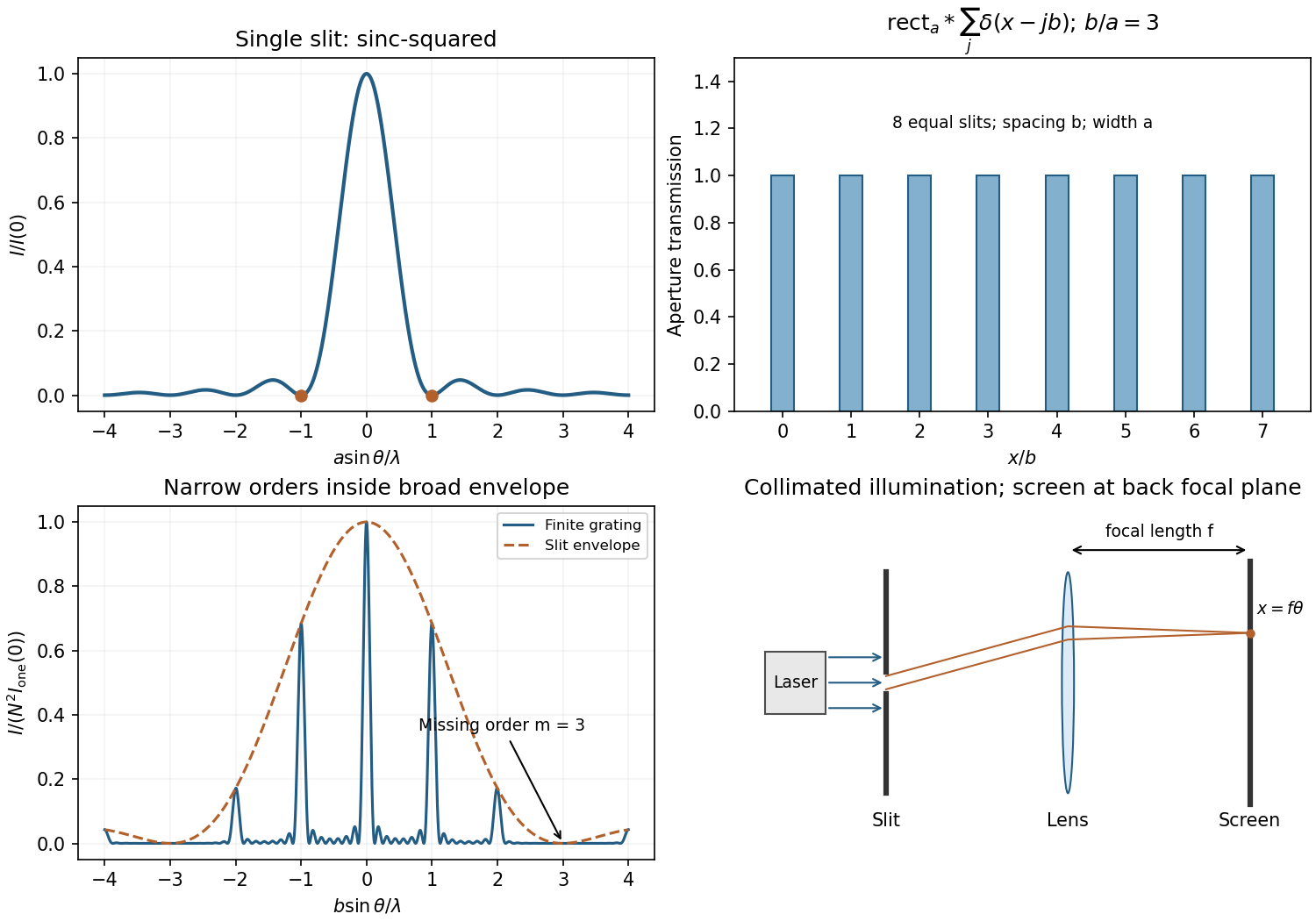
For uniform illumination, the aperture is $h(x)=1$ for $|x|<a/2$ and zero otherwise. With $q=2\pi \sin \theta /\lambda$,Zeros occur at $\sin \theta =j\lambda /a$, $j\ne 0$; the central maximum extends between $\pm \lambda /a$. A monochromatic laser expanded into a collimated beam can illuminate the slit. A lens with the screen in its back focal plane produces the Fraunhofer pattern; alternatively use a sufficiently distant screen, $z\gg a^2/\lambda$. Align the slit and beam and avoid detector saturation.

For $N$ equally spaced slits, write the aperture as a convolutionThe convolution theorem converts this into a single-slit transform times the finite-array transform. ThereforePrincipal maxima are at $b\sin \theta =m\lambda$ for normal incidence, inside the single-slit envelope. Their height scales as $N^2$ times the envelope, and their first zeros are separated from a peak by $\delta (\sin \theta )=\lambda /(Nb)$.

The envelope-to-order-spacing ratio is $b/a$: increasing it admits more orders within the central envelope and changes the relative order strengths. In particular, an order is missing when $ma/b$ is a nonzero integer. Statements about absolute angular spacing need a fixed dimension: at fixed $a$, increasing $b$ reduces order spacing; at fixed $b$, decreasing $a$ broadens the envelope.

For fixed incident angle, differentiating the grating equation gives an order displacement $\delta (\sin \theta )=|m|\delta \lambda /b$. Equating this to the peak-to-first-zero width givesHere $W\simeq Nb$ is the illuminated grating width; this is the ideal Rayleigh limit, before slit width or aberrations broaden the spectral image.

With $b=(1600\mathrm{m}{\mathrm{m}}^{-1}{)}^{-1}=0.000625\mathrm{mm}$, the required count is $N\ge 372.7/(2\times 0.2)=931.75$. Thus 932 illuminated slits, or $W_{\min }\simeq 0.5825\mathrm{mm}$, suffice ideally. Checking diffraction-order feasibility, normal incidence cannot produce this second order because $2\lambda /b=1.193>1$; an oblique spectrograph geometry is required. A feasible reflection-Littrow example has $\sin \theta =m\lambda /(2b)=0.5963$, or $\theta \simeq 36.6^{\circ }$.

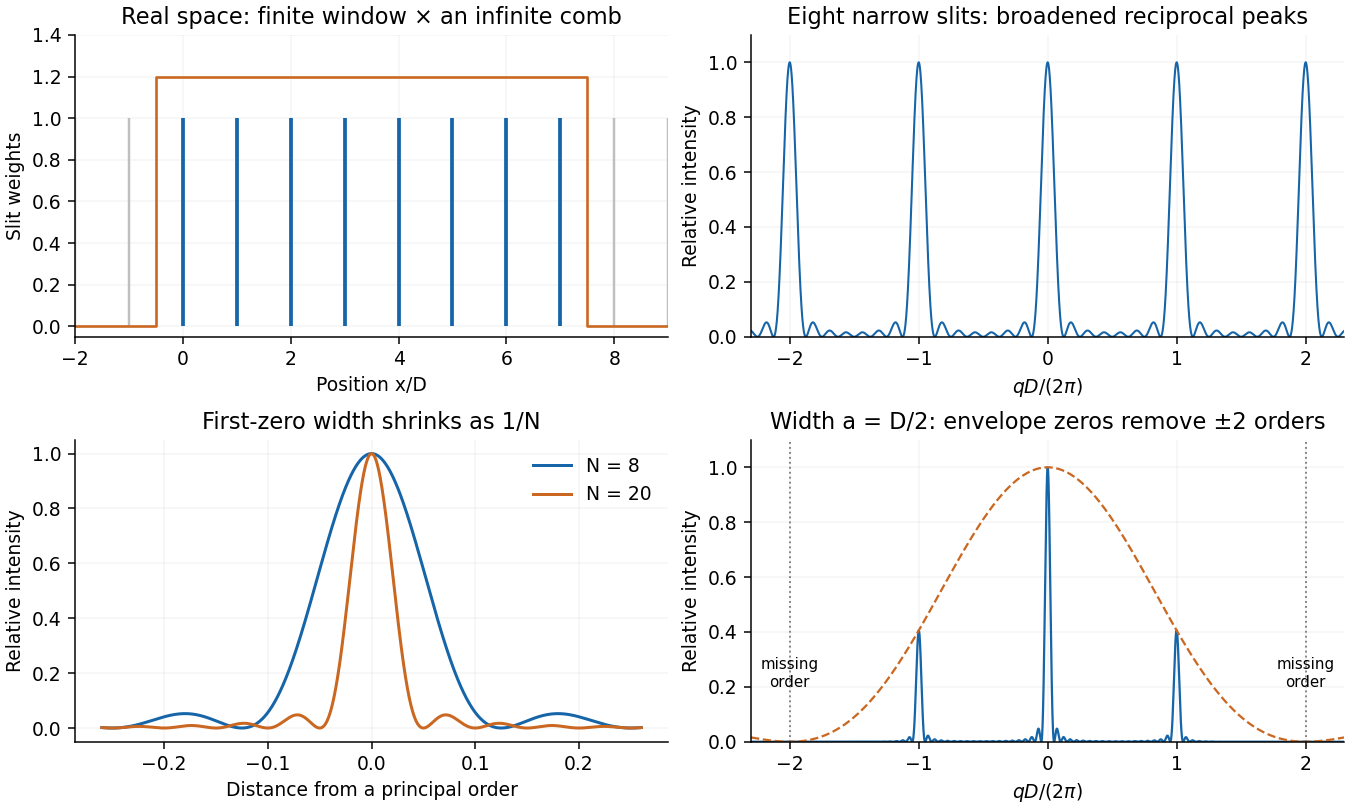
Use Fourier transform convention $\hat{f}(q)=\int f(x)e^{-iqx}dx$. The convolution theorem givesA finite array of very narrow slits at $x=jD$, $j=0,\dots ,N-1$, has transmission proportional to ${\sum }_j\delta (x-jD)$. It can be constructed by multiplying an infinite Dirac comb by a finite window. The infinite comb transforms to a reciprocal comb; the finite window convolves each reciprocal peak with a narrow sinc-shaped amplitude. Thus increasing the illuminated length narrows each Fraunhofer diffraction peak.

The exact finite sum makes the argument quantitative:Its normalized intensity is $[\sin (NqD/2)/(N\sin (qD/2)){]}^2$. Principal maxima occur at $qD=2\pi m$; their first zeros are displaced by $|\Delta (qD)|=2\pi /N$. Replacing the ideal narrow slit by a finite slit function convolves the array in real space, multiplying this field by the single-slit Fourier transform. Field amplitudes are transformed and combined before their squared modulus is taken.

The convolution of two aperture functions in one dimension isWith Fourier transform convention $\hat{f}(q)=\int f(x)e^{-iqx}dx$, the convolution theorem statesThe first identity follows by substituting the convolution integral, putting $v=x-u$, and separating the resulting double integral into $\int f(u)e^{-iqu}du$ times $\int g(v)e^{-iqv}dv$. For an absolutely integrable pair the interchange is justified by absolute convergence; finite optical apertures satisfy suitable integrability assumptions.

In Fraunhofer diffraction, the observed field is the Fourier transform of the transmitted complex aperture field. For two identical slits, let $g(x)$ be one slit and use a pair of Dirac delta distributions to locate the centres:Consequently $\hat{t}(q)=2\hat{g}(q)\cos (qD/2)$. For a rectangular slit, $\hat{g}=a\mathrm{sinc}(qa/2)$, giving a single-slit diffraction envelope times the double-slit interference factor in intensity. A $\pi$ phase reversal replaces the plus between the deltas by a minus, giving $\sin (qD/2)$ instead, as in B7.

More generally, an $N$-slit array is a single-aperture function convolved with a finite comb. Its field contains the factorThis separates the narrow diffraction grating maxima from the individual-aperture envelope. The same reasoning holds in two transverse dimensions. Multiplying an existing aperture by an additional finite mask instead convolves their field transforms and can broaden features. These are operations on complex fields: intensity is the squared modulus of the final field and cannot generally be substituted into the field-level convolution theorem.

The far-field complex amplitude is the two-dimensional Fourier transform of the aperture amplitude transmittance, evaluated at transverse spatial frequencies $q_x=k{\ell }_x$, $q_y=k{\ell }_y$. The light intensity is proportional to the squared magnitude of this transform.

Use linearity to add the transforms of simpler aperture components, preserving their relative phases. A translated component acquires a complex exponential factor. Repeated identical openings can be expressed as the convolution of one opening with a sum of Dirac delta functions; the convolution theorem then factors the field into a single-opening transform and an array factor. Multiplying aperture functions instead convolves their transforms. These operations simplify complex apertures without repeatedly evaluating the full diffraction integral. It is the complex amplitudes, rather than their wave intensities, that are added for coherent illumination.

Convolution describes the response of a linear time-invariant system to an arbitrary input. If $h$ is its impulse response and $f$ its input,This is a weighted sum of responses to shifted impulses. For integrable functions the operation is commutative and associative. A causal system has $h(t)=0$ for $t<0$, restricting the integral to past inputs. With the Fourier convention $F(\omega )=\int f(t)e^{-i\omega t}dt$, the convolution theorem gives $G=HF$.

For example, an RC low-pass frequency response has $h(t)={\tau }_0^{-1}{e}^{-t/{\tau }_0}\Theta (t)$ and $H(\omega )=(1+i\omega {\tau }_0{)}^{-1}$, where $\Theta$ is the Heaviside step function. Fast input variations are smoothed. The same mathematics describes optical blurring by a point spread function and many other linear response measurements.

Deconvolution tries to recover $f$ from measured $g$ and known $h$. In noise-free data one formally sets $F=G/H$ where $H\ne 0$. Zeros of $H$ lose corresponding information; small values amplify measurement noise. If the measured spectrum is $G+N$, the direct estimate has error $N/H$, which can be very large at frequencies strongly suppressed by the instrument. An inverse is therefore not automatically unique or stable.

One regularized spectral deconvolution reconstruction isThis minimizes $|HF-G{|}^2+\lambda |F{|}^2$ at each frequency and limits noise amplification, at the cost of bias and lost resolution. Choosing the regularization requires assumptions about noise and the desired signal; deconvolution cannot restore components that the data do not determine without such additional information.

There are three independent nonfactorized momentum integrals, namely a tadpole integral, the three-line sunset diagram integral, and the five-line banana integral. The six displayed Feynman diagrams involve six complete integral expressions:The distinction between independent building blocks and their products removes an ambiguity in counting “different momentum integrals”. For the strict divergent-wave-function renormalization interpretation of ii, the graphs in c reduce to $T,T^2,B_5$, comprising three full integral expressions and two independent nonfactorized building blocks.

Make a Wick rotation and use $m>0$ to separate ultraviolet divergences from infrared divergences. Write $D_E(k)=1/(k^2+m^2)$, and let $T,B_r(P)$ be the Euclidean versions of the integrals above, with their harmless overall factors of $i$ removed. A spherical ultraviolet cutoff givesThus the one-vertex quartic graph is linearly divergent, and the one-vertex sextic graph is quadratically divergent as $T_{\Lambda }^2$.

For the other two building blocks, the spatial Fourier transform is especially transparent. The three-dimensional Euclidean scalar propagator isThe convolution theorem converts the $r$ parallel lines into $G(x{)}^r$. Angular integration gives, with a short-distance cutoff $a={\Lambda }^{-1}$,This is a different convenient cutoff regularization for the connected block; power-divergent coefficients depend on the cutoff convention, whereas the conclusions about powers and the presence of a kinetic logarithm do not. The sinc function is understood to be $1$ at $P=0$.

For $r=3$, the integrand starts as ${\rho }^{-1}+O(1)$, soIts divergent part is independent of external momentum. In particular,The finite difference and its finite derivative show why the pure three-line sunset diagram does not need a divergent wave-function renormalization in three dimensions.

For $r=5$, the small-distance Taylor expansion isConsequentlyIn particular, the nonzero $P^2\log \Lambda$ term requires a genuine divergent wave-function renormalization, in addition to the mass counterterm. The coefficients here refer to the displayed position-space cutoff and have not included Feynman-diagram symmetry factors or bare couplings.

The comparison with the superficial degree of divergence isThus the actual leading power agrees with $\omega$ in every case. The additional logarithms in products come from ultraviolet subdivergences, which uniform power counting alone does not resolve.

For $T{B}_3$ and $T^2{B}_3$, differentiation with respect to $P^2$ removes the logarithmic divergence of $B_3$, but leaves divergent factors $T$ or $T^2$ multiplying a finite, nonpolynomial function of $P^2$. These are subdivergent contributions, not new nonlocal counterterms: subtracting each tadpole diagram subdivergence and the momentum-independent $B_3$ subdivergence removes them. For example, in a factorized subtraction scheme $T{B}_3\mapsto (T-T_{\mathrm{div}})(B_3-B_{3,\mathrm{div}})$, and likewise for $T^2{B}_3$. The remaining $B_5$ kinetic logarithm explains the strict interpretation in ii. A dimensional regularization scheme can suppress power divergences; it does not invalidate this cutoff-based comparison with $\omega$.

For integrable functions $u,v$, the convolution theorem in the chosen convention isLet $F(s,y)$ be the Fourier transform of $f(\cdot ,y)$ in the horizontal coordinate. Transforming Laplace's equation givesFor $s\ne 0$, exclude the growing exponential and obtain $F(s,y)=2e^{-|s|y}/(1+s^2)$. At $s=0$, continuity in frequency gives $F(0,y)=2$; a constant zero-frequency transform is compatible with spatial decay of $f$.

By the transform pair in part (a), the inverse transform of $e^{-|s|y}$ is the Poisson kernel for the upper half-plane, $P_y(x)=y/[\pi (x^2+y^2)]$. ThusThe Poisson extension of exponential boundary data is harmonic, approaches the continuous boundary data and decays at spatial infinity. For uniqueness, apply the maximum principle for harmonic functions to the difference of two solutions on increasingly large half-discs: it is zero on the real boundary and uniformly small on the distant semicircle.

The displayed Poisson integral is the bounded harmonic function on the upper half-plane with continuous boundary values $f(x,0)=e^{-|x|}$. Taking a Fourier transform in $x$ reduces Laplace's equation to ${\hat{f}}_{yy}-s^2\hat{f}=0$, and the bounded solution has multiplier $e^{-y|s|}$. The convolution theorem gives the displayed expression. At frequency zero the transformed function is constant in $y$, not zero: its value is the total boundary integral, two.

The function decays uniformly as $x^2+y^2\to \infty$. For large $y$, use $P_y\le 1/(\pi y)$ and the boundary L1 norm two. When $y$ is bounded and $|x|$ is large, split the convolution into $|t|\le |x|/2$ and its complement: the kernel is small on the first part, and the exponential boundary value is uniformly small on the second. This also distinguishes spatial decay of the harmonic function from decay of its zero-frequency Fourier coefficient.