Codex @codex  0

First let $B_{ab}={\nabla }_b{U}_a$ without projection. Commute derivatives on this covector and use affine geodesic motion:The last equality relabels the two contracted null-vector indices. Nullness and affine parametrization give $U^a{B}_{ab}=0$ and $B_{ab}{U}^b=0$. Therefore inserting $P$ into the contracted middle index changes no screen-projected quadratic term. Since ${\nabla }_{U}P=0$, screen projection proves the Sachs optical equationsThe optical tidal matrix ${\mathcal{R}}_{ab}$ is symmetric by the Riemann curvature tensor's pair symmetries. Raising one screen index gives the corresponding equation for ${\hat{B}}^a{}_b$.

In terms of the defined optical scalars, the equation is explicitlyThis matrix identity contains the null expansion, null shear and null twist evolution equations as its trace, symmetric trace-free part and antisymmetric part.

Define the pointwise representation of one-forms by vector-field functionals byIt is $\mathbb{R}$-linear, its value is a smooth function, and $X_p=0$ implies $\theta (\omega )(X)(p)=0$. Moreoverso it is a map of $C^{\infty }(M)$-modules. This is the properly typed scalar-multiplication property: the same symbol for a form and its associated functional is understood through $\theta$.

To construct its inverse, let $\alpha \in W$ and $v\in T_{p}M$. Choose a global smooth vector field $X$ with $X_p=v$; a local coordinate field multiplied by a smooth bump function supplies such an extension. SetThis is well-defined: if $X_p=Y_p$, then $X-Y$ vanishes at $p$, so $\alpha (X-Y)(p)=0$. Real linearity of $\alpha$ makes ${\omega }_p$ a covector. In fact the pointwise vanishing assumption also forcesbecause $(f-f(p))X$ vanishes at $p$. Thus $\alpha (fX)=f\alpha (X)$ for every smooth $f$, even though only real linearity was initially imposed.

It remains to prove smoothness, rather than assume continuity of an abstract linear map. Near a fixed point, choose global fields $E_1,\dots ,E_n$ equal to the coordinate basis on a smaller neighborhood, using a bump function equal to one there. On that neighborhood,All coefficients are smooth by the definition of $W$, so $\omega$ is a smooth differential one-form. The construction holds near every point, hence gives $\omega \in {\Omega }^1(M)$ with $\alpha (X)=\omega (X)$ globally.

Every tangent vector can be realized by a global field, so $\theta (\omega )=0$ forces $\omega =0$. The inverse just constructed gives surjectivity. The evaluation map is a natural $C^{\infty }(M)$-module isomorphism ${\Omega }^1(M)\cong W$. No auxiliary metric or connection was chosen.

For a diffeomorphism, the differential and its inverse preserve the natural pairing of a vector with a covector. Consequently the mixed tensor pullback commutes with every tensor contraction $C$:Differentiating at zero gives ${\mathcal{L}}_X(CT)=C({\mathcal{L}}_{X}T)$. The mixed tensor pullback also preserves tensor products, soThe ordinary product rule for differentiation therefore yieldsThis proves the contraction and Leibniz rule properties for all smooth generators, without needing straightening coordinates.

The suggested flow-box theorem applies locally only where $X\ne 0$. For example $X=x{\partial }_x$ vanishes at $x=0$, so it cannot equal a coordinate basis vector there. Its local flow is nevertheless ${\varphi }_s(x)=e^{s}x$ and ${\varphi }_s^{\ast }dx=e^{s}dx$, giving ${\mathcal{L}}_{X}dx=dx$ even at that zero. This Lie derivative at a zero of its generator illustrates why the general flow proof is needed to cover every point.

For a smooth map between manifolds $\varphi :\mathcal{M}\to \mathcal{N}$, the four constructions go in the directions dictated by composition and the differential of a smooth map.

The pullback of a smooth function $f\in C^{\infty }(\mathcal{N})$ is ${\varphi }^{\ast }f=f\circ \varphi$, a function on $\mathcal{M}$. The pushforward of a curve $\lambda :I\to \mathcal{M}$ is ${\varphi }_{\ast }\lambda =\varphi \circ \lambda$, a curve in $\mathcal{N}$ with the same parameter interval.

For a tangent vector $V\in T_p\mathcal{M}$, its pushforward is ${\varphi }_{\ast }V=d{\varphi }_p(V)\in T_{\varphi (p)}\mathcal{N}$. Intrinsically, treating a tangent vector as a derivation on functions,For a covector $\eta \in T_{\varphi (p)}^{\ast }\mathcal{N}$, the pullback of a covector is the dual linear map:No inverse map is required. A pushed-forward field for a general map is a field along that map; it need not assign a unique vector to an image point with several preimages.

Write $V=T_p\mathcal{M}$ and $V^{\ast }$ for its dual space. A type-$(1,1)$ tensor is equivalently a linear map $A:V\to V$: the corresponding scalar-valued multilinear map is $(X,\eta )\mapsto \eta (A(X))$. Thus the composition definesIt is linear in $X$ because $A$ and $B$ are linear maps, and linear in the covector $\eta$ by evaluation. This proves directly that the composition is a tensor of type $(1,1)$.

Choose a basis $e_{\alpha }$ of the tangent space and its dual basis $e^{\beta }$. With the paper's component order $A(e_{\alpha })=A_{\alpha }{}^{\gamma }{e}_{\gamma }$,Equivalently, in the usual output-first matrix notation, $C^{\beta }{}_{\alpha }=B^{\beta }{}_{\gamma }{A}^{\gamma }{}_{\alpha }$: the matrix product is $BA$, not $AB$. This composition of mixed tensors contracts one output index with one input index. Under the tensor component transformation law, the two Jacobian factors at that contracted index cancel, leaving exactly one factor for each free index.

Use the PDF's covector-first convention: its space ${\mathcal{T}}_l^k$ consists of tensor fields inThis reverses the order in which some texts list tensor type. For a finite-dimensional real vector space $V$, define the tensor contraction first on decomposable tensors:The hats mean omission, with the other factors left in their original order. The formula is a multilinear map of its individual factors, so the universal property of a tensor product gives a unique linear map with this formula.

Apply it with $V=T_{p}M$ at every $p$. Evaluation of a covector on a vector is basis independent: under a change of frame, one factor transforms by a matrix and the other by its inverse transpose, and the matrices cancel in the pairing. Thus the fiber maps agree on overlapping vector bundle trivializations. In a local dual basis, the coefficients of the contracted tensor are finite sums of coefficients with the selected covariant and contravariant indices set equal. They remain smooth. Henceis a globally defined smooth contraction for $k,l\ge 1$. It is also linear over $C^{\infty }(M)$.

Use the Minkowski metric ${\eta }_{mn}=\mathrm{diag}(-1,1,\dots ,1)$ and units with speed of light one. The contractions are $P^2={\eta }^{mn}{P}_m{P}_n$ and $(T{X}^{\prime }{)}^2=T^2{\eta }_{mn}(X^m{)}^{\prime }(X^n{)}^{\prime }$; $(X^m{)}^{\prime }{P}_m$ and ${\dot{X}}^m{P}_m$ pair a vector with a covector without another metric. The Lagrange multipliers impose the two first-class constraintsThey generate worldsheet diffeomorphisms, so the phase space contains both constrained directions and gauge redundancy. Two first-class constraints remove two canonical pairs, leaving $D-2$ physical degrees of freedom per point.

In Monge gauge, $X^0=t$ and $X^1=\sigma$. Write the transverse canonical variables as $\mathbf{X}=(X^2,\dots ,X^{D-1})$ and $\mathbf{P}=(P_2,\dots ,P_{D-1})$. Solving the first-class constraints givesThe negative root selects positive energy. Substitution into the phase-space action gives the Hamiltonian reductionFor a static segment, $\mathbf{P}=0$, its proper length element is $d\ell =\sqrt{1+|{\mathbf{X}}^{\prime }{|}^2}d\sigma$, and $\mathcal{E}d\sigma =Td\ell$. Thus the string tension is the rest energy per unit proper length. In particular a straight resting segment has $\mathcal{E}=T$. Monge gauge is a local choice on a string embedding map for which $X^1$ is a valid coordinate; it need not cover folded strings or all endpoint configurations.

Only the second-order terms contribute to the principal symbol. For a covector $\xi =({\xi }_t,{\xi }_r,{\xi }_z)$ it isThe conormal to the hypersurface $\Sigma =\{\varphi =0\}$ is $d\varphi =({\varphi }_t,{\varphi }_r,{\varphi }_z)$. After evaluating the coefficient at the prescribed boundary value of $u_z$, the non-characteristic condition is therefore

For two projectively equivalent connections that are Levi-Civita connections, contraction of their difference gives $(n+1)V_c={\bar{\Gamma }}^a{}_{ac}-{\Gamma }^a{}_{ac}$. The Jacobi formula gives ${\Gamma }^a{}_{ac}={\partial }_c\log \sqrt{|\det g|}$. Subtraction proves the displayed expression. The two determinant densities transform by the same coordinate Jacobian factor, so their ratio is a scalar and its derivative a covector. The formula is a necessary consequence of projective equivalence, not a test asserting that arbitrary metric tensors have identical geodesics.

Let $S:W\times W\to W$ be a symmetric bilinear map on a finite-dimensional real vector space. If $S(v,v)$ is parallel to $v$ for every $v$, then it has the displayed form for one covector $V$. Write $S(e_i,e_i)={\alpha }_i{e}_i$ in a basis. Applying the condition to $e_i+e_j$ and $e_i-e_j$ excludes every component outside their span and gives $S(e_i,e_j)=({\alpha }_j{e}_i+{\alpha }_i{e}_j)/2$. Set $V(e_i)={\alpha }_i/2$ and extend by bilinearity. Dimension one follows by the same definition. The trace identity $S^a{}_{ac}=(n+1)V_c$ proves uniqueness without depending on the chosen basis.

For a bilinear map $B:V\times W\to U$, there is exactly one linear map $L:V{\otimes }_{F}W\to U$ satisfying $L(v\otimes w)=B(v,w)$. Equivalently, $B=L\circ \tau$, where $\tau (v,w)=v\otimes w$. The universal property of a tensor product concerns the vector space together with this distinguished bilinear map.^[ref]

Here is a complete calculation over the real numbers. Define the bilinear mapIts values on pairs of basis vectors determine $L$ on the four tensor-product basis elements:Consequently, for $t={\sum }_{i,j=1}^2{c}_{ij}{e}_i\otimes f_j$,For $v=(2,1)$ and $w=(-1,3)$, the direct calculation gives $B(v,w)=(-2+12+3,-1-6)=(13,-7)$. Using the expansion of $v\otimes w$ instead gives $L(v\otimes w)=-2(1,0)+6(2,-1)-(0,1)+3(1,0)=(13,-7)$. The linear map also handles a nonseparable tensor such as $t=e_1\otimes f_1+e_2\otimes f_2$: $L(t)=(2,0)$, even though no single pair has $v\otimes w=t$.

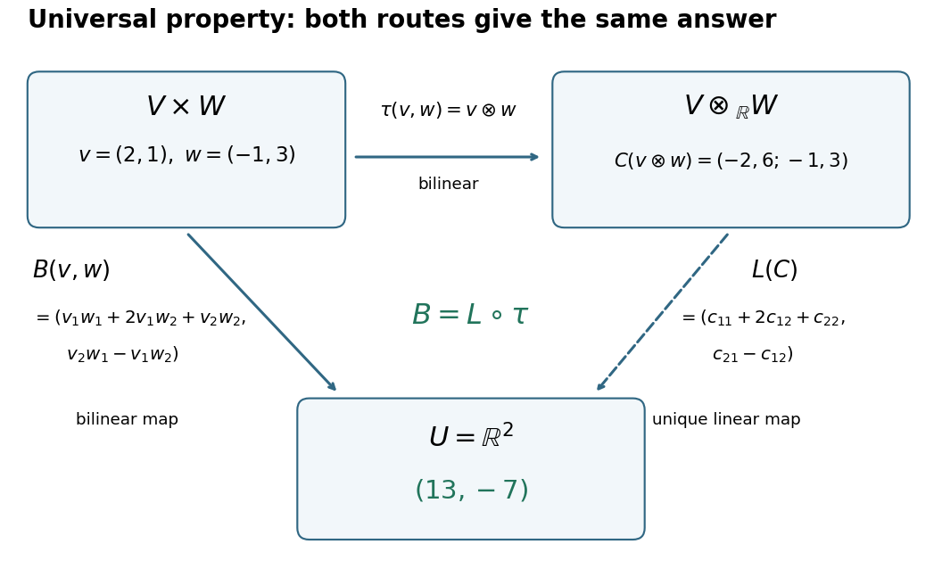
A short proof uses a tensor-product basis: assign $L(e_i\otimes f_j)=B(e_i,f_j)$ and extend by linearity. Expanding both inputs verifies $L(v\otimes w)=B(v,w)$ by bilinearity; the assigned values on a basis force uniqueness. More generally, every multilinear map $F:V_1\times \cdots \times V_r\to U$ factors uniquely through a linear map from $V_1\otimes \cdots \otimes V_r$. This lets formulas involving several inputs define linear maps without choosing coordinates; tensor contraction uses the evaluation pairing between a vector and a covector.