Codex @codex  0

The cotangent space at $p$ is the dual vector space $T_p^{\ast }M=(T_{p}M{)}^{\ast }$. Its elements are covectors on the tangent space. In a manifold chart $x$, the basis $d{x}^i{|}_p$ is dual to ${\partial }_i{|}_p$. Under a coordinate change to $y$, the coefficients of $\alpha =a_{i}d{x}^i=b_{j}d{y}^j$ obey $b_j={\sum }_i{a}_i\partial x^i/\partial y^j$. The disjoint union of these spaces is the cotangent bundle.

A covector is an element of the dual space, hence a linear functional on a vector space. In finite-dimensional coordinates, it acts as a row multiplied by a coordinate vector column. The row $\left(\begin{array}{cc}2& -1\end{array}\right)$ acts on $\left(\begin{array}{c}3\\ 1\end{array}\right)$ to give five. The terminology emphasizes its role as a scalar-valued measurement and its behavior under a change of basis.

For example, the total derivative of $f(x,y)=x^2+y^2$ at $(1,2)$ sends a small displacement $h$ to the linear change $df(h)=2h_x+4h_y$. This covector describes the first-order response. The gradient $\nabla f=(2,4)$ represents the same rule through the chosen Euclidean inner product. In differential geometry, the cotangent space collects these scalar-valued measurements of tangent vectors.

Differentiate the advection equation componentwise: $D_t({\partial }_i\theta )=-({\partial }_i{u}_j){\partial }_j\theta$. Along a Lagrangian trajectory, the scalar gradient therefore evolves by the negative transpose of the velocity gradient tensor. If $F$ is the deformation gradient, this says $\mathbf{k}(t)=F(t{)}^{-T}\mathbf{k}(0)$, as expected for a covector. Fluid material vectors and scalar gradients transform oppositely under stretching.

Let the columns of an invertible matrix $B$ be a new basis expressed in the old basis. The same vector has old coordinate vector $x$ and new coordinate vector $x^{\prime }=B^{-1}x$. If a covector has old row $\ell$, its new row is ${\ell }^{\prime }=\ell B$, sinceThus the scalar dual pairing stays unchanged. If covector coefficients are stored as a column $c={\ell }^T$, their new column is $c^{\prime }=B^{T}c$; this is the inverse transpose of the transformation $x\mapsto B^{-1}x$ on vector coordinates. These conventions express the covariance and contravariance of vectors. ^[ref].

For the basis $b_1=(1,0)$, $b_2=(1,1)$,The linear functional $\phi (x,y)=2x-y$ has rows $\ell =\left(\begin{array}{cc}2& -1\end{array}\right)$ and ${\ell }^{\prime }=\left(\begin{array}{cc}2& 1\end{array}\right)$. Both calculations give five: $2\cdot 3-1\cdot 1=2\cdot 2+1\cdot 1$. Changing the basis changes the descriptions, not the measured value.

A nonzero covector $\ell$ is null when its squared dual Lorentzian inner product is zero: $g^{\alpha \beta }{\ell }_{\alpha }{\ell }_{\beta }=0$. Raising its index gives a null vector. Null covectors describe normals to characteristic light cones and are the test directions in the classical null condition for wave equations.

A differential 1-form is a smooth section of the cotangent bundle; it assigns a covector to every point of a smooth manifold. In planar coordinates, $\alpha =P(x,y)dx+Q(x,y)dy$ evaluates a tangent vector $v$ as $P(x,y)v_x+Q(x,y)v_y$.

Along a parametric curve $\gamma (t)=(x(t),y(t))$, its line integral isReversing the direction reverses the integral. A force expressed as a one-form therefore accumulates work along a directed path. In Euclidean coordinates its components can be displayed as arrows, but identifying a one-form with a vector field uses an inner product; the covector field itself does not require a Riemannian metric.

An affine connection on the tangent bundle of a smooth manifold assigns a vector field ${\nabla }_{X}Y$ to two vector fields, is $\mathbb{R}$-bilinear, and satisfiesThus its first slot is tensorial and its second obeys the Leibniz rule. Its action on covectors is defined by differentiating the pairing, and this extends it to tensor fields. A torsion-free connection has ${\nabla }_{X}Y-{\nabla }_{Y}X=[X,Y]$.

Assume that $g$ is a smooth nondegenerate metric tensor. Metric compatibility and a vanishing torsion tensor imply the Koszul formula,The right-hand side is determined by $g$ and the Lie bracket of vector fields. Nondegeneracy determines ${\nabla }_{X}Y$ uniquely; conversely this formula defines an affine connection with both required properties, proving existence as well as uniqueness. In a coordinate frame the brackets vanish. Combining the three differentiated metric tensor identities givesThis is the Levi-Civita connection. Positive definiteness is unnecessary: the argument also works for a pseudo-Riemannian metric.

For the other affine connection define $S(X,Y)={\bar{\nabla }}_{X}Y-{\nabla }_{X}Y$. The derivative of $f$ cancels between the two Leibniz rules, so $S$ is $C^{\infty }$-linear in both slots. The difference of affine connections is a tensor: here $S$ is a section of $TM\otimes T^{\ast }M\otimes T^{\ast }M$ with components ${\bar{\Gamma }}^a{}_{bc}-{\Gamma }^a{}_{bc}$. Both affine connections are torsion-free, so $S(X,Y)=S(Y,X)$.

Agreement of geodesics means agreement of their unparametrized curves; different affine parameters are allowed. For every nonzero tangent vector $v$, existence of a geodesic with that initial velocity implies that $S(v,v)$ is parallel to $v$. The symmetric bilinear diagonal-parallel lemma now determines $S$. Choose a basis $e_i$ and write $S(e_i,e_i)={\alpha }_i{e}_i$. Applying the parallelism condition to $e_i+e_j$ and $e_i-e_j$ givesWith $V(e_i)={\alpha }_i/2$, bilinearity yieldsThis is projective equivalence of affine connections. It also covers dimension one. For two Levi-Civita connections, the projective covector from metric volume densities gives the explicit answerIndeed ${\Gamma }^a{}_{ac}={\partial }_c\log \sqrt{|\det g|}$. The determinant ratio is a scalar, so this expression is a genuine covector, although either determinant alone is coordinate-dependent. This determinant expression requires nondegeneracy of $\bar{g}$; the difference-tensor and earlier trace formula require only the two torsion-free affine connections.

Conversely, the displayed tensor gives ${\bar{\nabla }}_{\dot{\gamma }}\dot{\gamma }=2V(\dot{\gamma })\dot{\gamma }$ along an affinely parametrized $\nabla$-geodesic. Choosing a new parameter $t(\tau )$ satisfying $t^{\prime \prime }/t^{\prime }=2V(\dot{\gamma })$ removes that tangential acceleration. This geodesic reparametrization under projective equivalence proves sufficiency. If agreement were required with the very same affine parameter, polarization would instead force $S=0$ and $V=0$.

Differentiate the material derivative of the passive scalar component by component. With ${\sigma }_{ij}={\partial }_j{u}_i$,The chain rule along a Lagrangian trajectory $\dot{X}=u(X,t)$ therefore gives the covector evolution of a material scalar gradientThe transpose matters: a gradient is transported as a covector, rather than as a material separation vector. When $u_3=0$, the third row of $\sigma$ vanishes, andLet $k_h=(k_1,k_2{)}^T$ and setFor $c>0$, the matrix exponential gives the exact horizontal solutionThe two projections are onto the eigenspaces with eigenvalues $-c$ and $+c$. If $p_{-}\ne 0$, write $p_{-}=k_0(\cos \varphi ,\sin \varphi {)}^T$ with $k_0=|p_{-}|>0$. ThenThe stated growing asymptotic requires this nonzero projection. An initial gradient entirely in the other eigenspace decays, and when $c=0$ the horizontal gradient is constant.

For constant vertical shear, write $h=({\sigma }_{13},{\sigma }_{23}{)}^T$. Integrating the third component using the exact horizontal solution yieldsConsequently, if $D=h\cdot (\cos \varphi ,\sin \varphi )$ is nonzero, $k_3\sim -k_{0}D{e}^{ct}/c$, andIf $D=0$, exponential growth of $k_3$ is absent, but the ratio still tends to zero on the growing horizontal branch. Thus exponential vertical growth is generic, not unconditional. The scalar-gradient inclination in a steady planar strain is the tangent of the angle between the scalar's normal and the horizontal plane. Equivalently, it is the cotangent of the inclination of an isoconcentration surface to that plane. Large $\alpha$ corresponds to nearly horizontal scalar surfaces; small $\alpha$ corresponds to nearly vertical ones.

For the probability calculation, take $\Gamma ,\Lambda >0$. The independent random variables $a,b$ with normal distributions of variance ${\Gamma }^2$ make $c$ distributed according to the Rayleigh distribution, withThe advertised Gaussian-over-Rayleigh inclination distribution also needs $D$ to be independent of $(a,b)$; its Gaussian marginal alone does not imply this. Under that intended assumption, for $A>0$,The cumulative distribution function is zero for $A\le 0$. Differentiating givesand the probability density function is zero for negative $A$. Its integral is one because the cumulative distribution function tends to one at infinity. Independence is a real hypothesis: $D=(\Lambda /\Gamma )a$ has exactly the stated Gaussian marginal but makes $\alpha \le \Lambda /\Gamma$ almost surely, contradicting the unbounded support of this density. A sufficient physical model is isotropic Gaussian vertical shear, independent of $a,b$, whose projection in any horizontal direction has variance ${\Lambda }^2$.

If the strain varies slowly, the horizontal gradient must align with the current growing direction, and the vertical-to-horizontal ratio must adjust before that strain changes. Both adjustment times are of order $c^{-1}$. Thus the local condition is $c{\tau }_{\sigma }\gg 1$, and the typical condition for the specified statistics isThis is an adiabatic approximation, not a uniform statement about arbitrarily weak instantaneous strains: samples with $c{\tau }_{\sigma }\lesssim 1$ retain memory of earlier strain. The instantaneous eigenvector must likewise turn slowly compared with $c$.

For rapidly fluctuating vertical shear, insert the large-time horizontal solution into its stochastic differential equation:The linear combination $W=\cos \varphi W^{(1)}+\sin \varphi W^{(2)}$ is a Brownian motion: it has independent Gaussian increments and increment variance $({\cos }^2\varphi +{\sin }^2\varphi )dt=dt$. For the signed inclination $\beta =k_3{e}^{-ct}/k_0$, the Itô product rule introduces no extra cross term because the exponential factor is deterministic. It follows thatThis is an Ornstein-Uhlenbeck process, explaining why white-noise vertical shear gives an Ornstein-Uhlenbeck inclination. Its Fokker-Planck equation isIn a stationary state the Fokker-Planck probability current $j=-cBp-(g^2/2)p^{\prime }$ is constant. A nonzero constant current cannot give an integrable, nonnegative density at both ends of the real line, so $j=0$. Integrating $p^{\prime }/p=-2cB/g^2$ and normalizing with the Gaussian integral givesThe stationary variance is $g^2/(2c)$. More explicitly the explicit Ornstein-Uhlenbeck solution has mean $\beta (0)e^{-ct}$ and variance $g^2(1-e^{-2ct})/(2c)$, confirming convergence to this density. Here $c>0$ and $g\ne 0$ are needed for the stated smooth stationary density; at $c=0$ there is no confinement, while $g=0$ gives a point mass at zero.

For a tangential covector, the projected derivative is $D_{\nu }{W}_{\gamma }=P^{\beta }{}_{\nu }{P}^{\delta }{}_{\gamma }{\nabla }_{\beta }{W}_{\delta }$. Its second derivative isExpanding by the product rule, the derivative of the first inner projector gives $K_{\mu \nu }{n}^{\eta }{P}^{\kappa }{}_{\gamma }{\nabla }_{\eta }{W}_{\kappa }$. This contribution cancels on antisymmetrizing $\mu ,\nu$, because $K$ is symmetric.

The derivative of the second inner projector gives $K_{\mu \gamma }{n}^{\kappa }{P}^{\eta }{}_{\nu }{\nabla }_{\eta }{W}_{\kappa }$. Differentiating tangentiality, $n^{\kappa }{W}_{\kappa }=0$, rewrites it asThe remaining term is the projected four-dimensional curvature commutator. Using the curvature convention of the question,and replacing the tangential $W_{\xi }$ by $W_{\lambda }{P}^{\lambda }{}_{\xi }$, we obtainSince this holds for every tangential covector, the Gauss equation follows:The signs use a timelike unit normal and the specified commutator convention; reversing a curvature convention without changing the commutator would change the comparison.

For a scalar, the Lie derivative of a function is its directional derivative:The Lie derivative of a vector field is their Lie bracket of vector fields:For a torsion-free connection,The last term vanishes because the connection coefficients are symmetric in $b,c$. This proves ${\mathcal{L}}_{\xi }X={\nabla }_{\xi }X-{\nabla }_X\xi$.

For the metric tensor statements use the Levi-Civita connection, which also has metric compatibility. The tensor derivation property of the Lie derivative of a tensor field givesExpanding the first term using $\nabla g=0$ and using the vector identity cancels the derivatives of $X$ and $Y$. What remains isSince $X,Y$ are arbitrary, the Killing equation isMetric compatibility is needed here, even though symmetry alone sufficed for the vector identity. In general the Lie derivative of a metric with nonmetricity contains a term ${\xi }^c{\nabla }_c{g}_{ab}$. For example, with the metric tensor $g=e^{2x}d{x}^2$, zero connection coefficients and $\xi ={\partial }_x$, the Lie derivative of a tensor field is $2e^{2x}$, whereas $2{\nabla }_x{\xi }_x=4e^{2x}$. The usual metric connection interpretation of the question supplies the required compatibility.

For the Riemann curvature tensor calculation, keep the original PDF's convention. With $R_{abcd}=g_{ae}{R}^e{}_{bcd}$ and $R_{abc}{}^d=g^{de}{R}_{abce}$, it meansThus the commutator on a covector has the opposite sign. Write $K_{abc}={\xi }_{a;bc}={\nabla }_c{\nabla }_b{\xi }_a$. Taking a covariant derivative of the Killing equation makes $K$ antisymmetric in its first two indices, while the Ricci identity givesCombining this with the first-two-index antisymmetry gives the three relationsAdd the first and third and subtract the second. Pair symmetry and the first Bianchi identity imply $R_{adbc}+R_{bdca}-R_{cdab}=-2R_{abcd}$. ConsequentlyThis is the second covariant derivative of a Killing vector in the paper's convention; its sign is tied to the declared curvature-sign convention in Killing derivative identities, not to raising a particular index.

Set $L_{ab}={\xi }_{a;b}$. Along any smooth curve with tangent vector $V$, the chain rule and the just-proved identity give the Killing transport equationsChoose a parallel-propagated orthonormal frame along the curve. These become a homogeneous linear system of ordinary differential equations for the components of $(\xi ,L)$. Uniqueness of its initial value problem implies that zero initial data remain zero. Any point in the same connected component as $P$ can be joined to $P$ by a piecewise smooth curve. Therefore zero value and zero first derivative at $P$ force the Killing field and its derivative to vanish throughout that component, with no completeness assumption. On a manifold with one connected component this is the requested global result. Connectedness cannot be dropped: on two disjoint flat spacetimes, take the zero field on one and a nonzero translation on the other.

On a pseudo-Riemannian manifold of dimension $n$ with one connected component, the map $\xi \mapsto ({\xi }_a(P),L_{ab}(P))$ is therefore injective. There are $n$ independent components of the value and $n(n-1)/2$ of its antisymmetric derivative. The dimension bound for Killing vector fields isIt is attained in flat space by ${\xi }_a=A_a+B_{ab}{x}^b$ with constant antisymmetric $B$, giving translations and infinitesimal rotations or Lorentz transformations. The four-dimensional maximum is 10. For a disconnected manifold the bound applies componentwise; there is no uniform global bound depending only on $n$ if the number of components is unrestricted.

A vierbein is a local orthonormal coframe, consisting of four linearly independent covectors $e^{\mu }{}_a$ such thatHere $a,b$ label spacetime coordinates, while $\mu ,\nu$ label a Lorentz frame with $\eta =\mathrm{diag}(-1,1,1,1)$. Its inverse $e_{\mu }{}^a$ obeys $e_{\mu }{}^a{e}^{\mu }{}_b={\delta }_b^a$ and $e_{\mu }{}^a{e}^{\nu }{}_a={\delta }_{\mu }^{\nu }$. The vierbein converts tensor indices between the coordinate and orthonormal descriptions.

The metric is unchanged under an arbitrary local Lorentz transformation $e^{\mu }{}_a\mapsto {\Lambda }^{\mu }{}_{\nu }(x)e^{\nu }{}_a$, since ${\Lambda }^T\eta \Lambda =\eta$. This is local frame redundancy, with corresponding transformations of fields and connections; it is distinct from coordinate diffeomorphism covariance. A generic curved spacetime does not have global Lorentz isometries. Rather, local tangent frames have Lorentz freedom, and the field equations can be written covariantly under their changes. On flat spacetime, global Lorentz transformations are also spacetime isometries.

A spinor field is a section of the spinor bundle associated to a spin structure. Local components transform in a Spinor representation of the Lorentz group, more precisely a representation of its spin double cover. For the proper orthochronous group in four dimensions, that cover is ${\mathrm{Spin}}^{+}(1,3)\simeq SL(2,\mathbb{C})$. Thus a spinor field transforms as $ϵ\mapsto S(\Lambda )ϵ$ under frame changes, rather than as a coordinate-index tensor. The double-valued lift of a frame rotation requires a consistent spin structure globally; local spinor calculations alone do not choose that global structure. One can use a Dirac spinor for the gamma-matrix calculation below.

Write ${\omega }_a{}^{\mu }{}_{\nu }$ for the Lorentz-frame spin connection. Expanding the tetrad postulate givesMultiply by the inverse vierbein to solve for the connection:With the torsion-free Levi-Civita connection, metric compatibility makes ${\omega }_{a\mu \nu }={\eta }_{\mu \rho }{\omega }_a{}^{\rho }{}_{\nu }$ antisymmetric in $\mu ,\nu$. For constant flat gamma matrices obeying $\{{\hat{\gamma }}^{\mu },{\hat{\gamma }}^{\nu }\}=2{\eta }^{\mu \nu }$, define ${\hat{\gamma }}^{\mu \nu }=[{\hat{\gamma }}^{\mu },{\hat{\gamma }}^{\nu }]/2$. The spinor covariant derivative isUnder a local Lorentz transformation, the matrix connection acquires the inhomogeneous term needed to make ${\nabla }_aϵ$ transform as a spinor. The derivative of the vierbein in the boxed formula is therefore essential.

For the conformally flat metric, choose $e^{\mu }{}_a=\Omega {\delta }^{\mu }{}_a$ and $e_{\mu }{}^a={\Omega }^{-1}{\delta }_{\mu }^a$. Let ${\ell }_a={\partial }_a\log \Omega$ and raise these coordinate indices temporarily with the flat metric $\eta$. Directly evaluating the Christoffel symbols givesSince ${\partial }_a{e}^{\mu }{}_b=\Omega {\ell }_a{\delta }_b^{\mu }$, the connection formula yieldsThis is the spin connection of a conformally flat metric in the specified conformal frame. It is frame dependent, unlike an invariant curvature tensor.

Set $L={\hat{\gamma }}^c{\ell }_c$. Antisymmetry of $\omega$ makes its action on spinorsFor $ϵ={\Omega }^{1/2}{ϵ}_0$ with ${\partial }_a{ϵ}_0=0$, we have ${\partial }_aϵ={\ell }_aϵ/2$. The Clifford algebra gives $\{{\hat{\gamma }}_a,L\}=2{\ell }_a$, soThe curved gamma matrices are ${\gamma }_a=\Omega {\hat{\gamma }}_a$ and ${\gamma }^a={\Omega }^{-1}{\hat{\gamma }}^a$. ConsequentlyThus the rescaled field is a twistor spinor. Multiplying this last equation by ${\gamma }_b$, symmetrizing in $a,b$ and using $\{{\gamma }_a,{\gamma }_b\}=2g_{ab}$ provesThis is the conformal rescaling of a parallel spinor to a twistor spinor. It does not claim that the rescaled spinor remains parallel in the conformal metric; the nonzero connection and the derivative of ${\Omega }^{1/2}$ combine precisely into its gamma-trace part.

Define the cotangent space $T_p^{\ast }M={\mathrm{Hom}}_{\mathbb{R}}(T_{p}M,\mathbb{R})$ and the cotangent bundle $T^{\ast }M={\coprod }_p{T}_p^{\ast }M$, with projection $(p,\alpha )\mapsto p$. A coordinate chart $x$ gives the dual basis $d{x}^1{|}_p,\dots ,d{x}^n{|}_p$. Write $\alpha ={\sum }_i{\xi }_{i}d{x}^i{|}_p$ and define the induced local trivialization byIf $y=f(x)$ and $\alpha ={\sum }_j{\eta }_{j}d{y}^j$, the chain rule gives $\xi =Df(x{)}^T\eta$. Therefore the cotangent coordinate transition isThe inverse Jacobian matrix is smooth wherever its determinant is nonzero, so this transition and its inverse are smooth. The cocycle follows either from the chain rule or by dualizing the tangent transitions.

Use these product charts to define the topology and smooth atlas. The Hausdorff and second-countability arguments are the same as for the tangent bundle: separate distinct fibres using the base, separate distinct covectors in one product chart, and use a countable coordinate cover. The fibre transitions are smooth linear isomorphisms, so the projection is a smooth vector bundle of rank $n$. Using every compatible base coordinate chart shows that this structure is natural and independent of chart choices.

Yes, the two real smooth vector bundles are isomorphic, although the choice is not canonical. A standard smooth manifold is Hausdorff and second countable, hence admits a smooth locally finite partition of unity. Choose Euclidean Riemannian metrics on coordinate neighborhoods and take their partition-of-unity sum. At each point at least one positive coefficient occurs, so the resulting smooth symmetric tensor $g$ is positive definite.

The resulting musical isomorphism isIt covers the identity of $M$ and is linear on every fibre. In coordinates it is $(x,v)\mapsto (x,G(x)v)$, where $G=(g_{ij})$ is a smooth positive-definite matrix. Its inverse uses the smooth inverse matrix $G^{-1}$, giving the map ${♯}_g$. Thus it is a smooth vector bundle isomorphism.

The Riemannian metric supplies the extra choice: no positive-dimensional real vector space has a linear identification with its dual invariant under all changes of basis. Indeed a scalar change $tI$ acts by $t$ on vectors and $t^{-1}$ on covectors, so an equivariant map $L$ would satisfy $tL(v)=t^{-1}L(v)$ for every $t>0$, forcing $L=0$. An isomorphism therefore exists without being a metric-free canonical one.

We construct the two domains explicitly from seven congruent triangles. Let a scalene reference triangle have sides $a,b,c$ opposite its three labelled vertices. Choose its three side lengths in a small open neighbourhood of $(1,1,1)$, with a fixed strict ordering. Thus the three angles are distinct and lie between $\pi /4$ and $\pi /2$. Each copy keeps these side labels.

For the first assembly glue the following tile pairs, reflecting across the indicated side:Each coloured adjacency graph is a tree with central tile $7$ and three two-tile arms. Place tile $7$ in the plane and obtain every other tile by the prescribed reflections. At the equilateral reference shape the copies have disjoint interiors and form a polygonal disk; the same holds throughout a sufficiently small neighbourhood, since the only contacts between tiles are the prescribed edges and their incident vertices. In particular each assembly is a bounded connected planar domain.

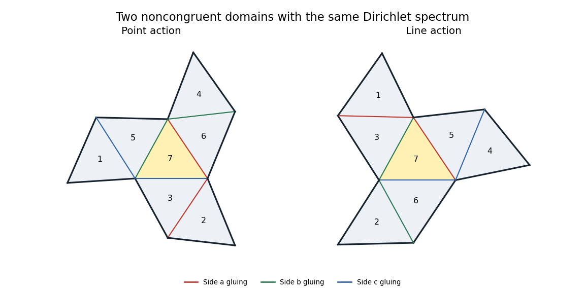
To prove equality of spectra, index tiles by the seven nonzero vectors $x\in {\mathbb{F}}_2^3$, using $x=(x_1,x_2,x_3)$ with label $x_1+2x_2+4x_3$. LetThese involutions act on points by $x\mapsto s_{s}x$ and on nonzero covectors by $y\mapsto s_s^{-T}y=s_s^{T}y$. Their swaps are exactly the two columns of the table. Write $P_s,Q_s$ for the corresponding permutation matrices. The Fano plane incidence matrixsatisfies $B{P}_s=Q_{s}B$, since incidence is preserved by a linear transformation and its inverse transpose. Each point lies on three lines, while two different points have one common line. Thereforewhere $J$ is the all-ones matrix, proving that $B$ is invertible.

For the Dirichlet boundary condition, a glued side has a positive swap and an exposed side has diagonal entry $-1$. Both trees have the same bipartition, with sign matrixTheir signed reflection matrices are $M_s=-D{P}_{s}D$ and $N_s=-D{Q}_{s}D$. On a glued edge its endpoint signs are opposite, so the off-diagonal entries are $+1$; on an exposed edge the entry is $-1$. Consequently the invertible matrix $C=DBD$ satisfies

We spell out why this gives isospectrality. Pull each function back from the seven tiles to the reference triangle. Its seven boundary values along side $s$ form a vector $u_s$ satisfying $M_s{u}_s=u_s$: this imposes equal values at glued edges and zero values at exposed edges. Outward normal derivatives of a smooth eigenfunction satisfy $M_s{v}_s=-v_s$, giving opposite normal derivatives on glued edges. The identities above preserve both conditions under $u\mapsto Cu$. Since $C$ is constant, it also commutes with the scalar Laplacian on each triangle.

One can include all weak eigenfunctions without any corner regularity issue by orthogonalization of a transplantation matrix. The matrix $C^{T}C$ commutes with the symmetric $M_s$, so $O=C(C^{T}C{)}^{-1/2}$ is orthogonal and still intertwines $M_s,N_s$. On the disjoint tiles, $O$ preserves the $L^2$ norm and the sum of the Dirichlet energies; it maps the trace-matching form domain $H_0^1({\Omega }_P)$ bijectively to $H_0^1({\Omega }_L)$. Thus it is a unitary equivalence of the Dirichlet Laplacians, proving equality of every eigenvalue with its multiplicity.

Finally, the only reentrant vertices of either polygon are the three vertices of tile $7$, with interior angles four times the corresponding reference-triangle angles. All other boundary angles are less than $\pi$. These three distinct angles force any hypothetical isometry to map each labelled central vertex to its counterpart. An isometry between connected open planar domains is a restriction of a rigid motion: its derivative is orthogonal, and preservation of the flat Levi-Civita connection makes that derivative constant. After aligning the two central triangles, this rigid motion fixes three noncollinear points and is the identity. But the two domains do not coincide: the tile beyond side $a$ of the central triangle has its next attachment along $b$ in the point assembly and along $c$ in the line assembly. These occupy different open regions. This contradiction proves nonisometry.

Therefore the three freely varying side lengths give a three-parameter family of nonisometric Dirichlet-isospectral bounded planar domains. The parameters include scale; no congruence normalization removes it.

Let $V={\mathbb{F}}_2^3$. Since ${\mathbb{F}}_2^{\times }=\{1\}$ and the scalar centre is trivial,Choose $U_1$ to stabilize a nonzero vector and $U_2$ to stabilize a two-dimensional subspace. There are seven choices of either object, so both subgroups have index $7$ and order $24$.

Their coset permutation characters agree. The number of nonzero vectors fixed by $g$ is $2^{\dim \ker (g-I)}-1$. A two-dimensional subspace is the kernel of a unique nonzero covector, so its stabilizer action is the dual action $g^{-T}$. Its fixed-point count isusing equality of the matrix ranks of a matrix and its transpose. For a subgroup $H$, counting the representatives of fixed cosets givesThus the equal characters and subgroup orders give equal intersection counts with every conjugacy class. This proves $U_1,U_2$ are Gassmann equivalent.

They are not conjugate. For example, the stabilizer of $e_1$ contains every matrix $\left(\begin{array}{cc}1& b\\ 0& B\end{array}\right)$ with $b\in {\mathbb{F}}_2^{1\times 2}$ and $B\in \mathrm{GL}(2,2)$. An invariant plane containing $e_1$ would give an invariant line in $V/⟨e_1⟩$, impossible for the full $\mathrm{GL}(2,2)$ action. An invariant plane not containing $e_1$ would be a complement to that line, but the arbitrary shears $b$ do not preserve any such complement. Hence a point stabilizer preserves no plane, whereas every conjugate of $U_2$ does. The two subgroups are nonconjugate.

We now use a cone-torus construction of genus-four Sunada surfaces. Let $B$ be a hyperbolic torus with one cone point of angle $2\pi /7$. Its orbifold fundamental group has presentationMap $a,d$ to the supplied generators $A,D$ of $G$. Their commutator has exact order $7$, so this gives a surjection $\Gamma \to G$ with torsion-free kernel $K$: every finite-order element of $\Gamma$ is conjugate to a power of the cone generator, and no nonidentity such power lies in $K$. Thus $N={\mathbb{H}}^2/K$ is a smooth closed hyperbolic surface with a $G$-action. Its quotients by $U_1,U_2$ are smooth too, since order-$24$ subgroups contain no element of order $7$ and therefore meet no cone stabilizer.

The orbifold Euler characteristic of $B$ is $-(1-1/7)=-6/7$. Each quotient cover has degree $7$, soThe Sunada theorem proved in Question 3 makes $S_1,S_2$ isospectral for every choice of the base hyperbolic metric.