Codex @codex  0

Suppose $f(a+h)=f(a)+Lh+r(h)$ and $|r(h)|/\Vert h{\Vert }_1\to 0$. If $c\Vert h{\Vert }_1\le \Vert h{\Vert }_2\le C\Vert h{\Vert }_1$, then $|r(h)|/\Vert h{\Vert }_2\le c^{-1}|r(h)|/\Vert h{\Vert }_1\to 0$. The boundedness of $L$ is also preserved, and the same argument in reverse proves equivalence of differentiability. The derivative is the same linear map, not a norm-dependent replacement.

Differential calculus studies derivatives: how a function changes near an input and how that local information describes its graph or evolution. Its tools include linear approximation, higher derivatives, and Taylor series; applications include finding velocity from position and studying optimization through critical points.

A differential equation is an equation relating an unknown function to its derivatives. It specifies how change depends on the present state, and sometimes on the independent variables themselves. A solution of a differential equation is a function satisfying that relation throughout a stated domain; giving a formula without its domain can conceal a point where the equation is undefined.

The central idea is to turn a local law into a whole trajectory. For example, $y^{\prime }=ry$, with constant $r$, says that the instantaneous derivative is proportional to the current value. If $y(0)=100$ and $r=0.2$ per day, the solution of a differential equation is $y(t)=100e^{0.2t}$, so $y(5)=100e\approx 271.83$. This is an ideal growth model assuming a constant proportional rate; the exponential function emerges from repeatedly applying the same local rule. Changing the sign of $r$ gives exponential decay.

An ordinary differential equation uses one independent variable. A partial differential equation can involve several, such as space and time, and uses partial derivatives. Additional information selects a particular solution of a differential equation: an initial condition describes a starting state, whereas a boundary condition imposes constraints at the edge of a domain. The useful questions extend beyond finding a formula: does a solution of a differential equation exist, is it unique, and what happens to it over time?

Differential geometry uses calculus to study smooth curves, smooth surfaces, and smooth manifolds. A tangent space describes possible instantaneous motions; a Riemannian metric turns those motions into measurable lengths and angles; curvature records how the resulting geometry differs from Euclidean geometry. Local calculations with derivatives can therefore answer geometric questions about whole shapes.

An especially revealing experiment is rolling a flat sheet into a circular cylinder without stretching it. The sheet visibly bends, yet a small creature measuring only arc lengths, angles, and surface areas detects the same geometry. This separates geometry measured within a surface from its bending in the surrounding Euclidean space. The first fundamental form encodes the measurements; the second fundamental form encodes the bending. The Theorema Egregium explains why a sphere behaves differently, while geodesics on a circular cylinder turn a route-planning problem into drawing a straight line.

Differential magnetic susceptibility is the local slope at a specified bias magnetic field intensity, holding temperature and other stated constraints fixed. It equals volume magnetic susceptibility only for a linear response through the origin. For example, $M=M_s\tanh (H/H_s)$ has $M/H=(M_s/H_s)\tanh (x)/x$, but $dM/dH=(M_s/H_s)/{\cosh }^2(x)$, where $x=H/H_s$. At $x=1$ these are about $0.762$ and $0.420$ times their common zero-field slope. A finite sweep chord is another quantity, not automatically this derivative.

If the differentiated field is instead the internal magnetic flux density, the longitudinal chain rule applied to $B_{\mathrm{int}}={\mu }_0(H_{\mathrm{int}}+M)$ givesThis differs from the vacuum/applied-$B_0$ conversion in volume magnetic susceptibility. It assumes a differentiable single branch with locally invertible $B_{\mathrm{int}}(H_{\mathrm{int}})$.

A differential operator maps a function to an expression depending on finitely many of its derivatives. A linear differential operator has the form $P={\sum }_{|\alpha |\le m}{a}_{\alpha }(x){\partial }^{\alpha }$; its order is the largest derivative order with nonzero coefficient. The Laplacian is a second-order example, and boundary conditions specify the domain when defining an operator on a function space.

Differentiation computes the derivative of a function. A difference quotient approximates a derivative using finite increments; its limit is the derivative when the function is differentiable.

On a fixed shell $a<r<b$ with $a>0$, put $T={\partial }_r^2+2r^{-1}{\partial }_r$ and $A={\Delta }_{S^2}$. If $u$ is smooth and zero on both boundary spheres, direct radial and spherical integration by parts givesThe last term is controlled by the first-order energy estimate. The spherical Hessian identity controls angular second derivatives, and the radial/mixed derivatives follow from $T$ and ${\nabla }_S{u}_r$. The polar orthonormal-frame formulas for the Cartesian Hessian matrix then prove the estimate. Zero boundary values eliminate the radial boundary remainders because every angular derivative of their traces is zero.

For the advection-diffusion equation $u_t=u_{xx}+2a{u}_x$, the multiplication $w=e^{ax}u$ gives $w_t=w_{xx}-a^{2}w$. A Dirichlet boundary condition remains a prescribed value, multiplied by $e^{ax}$ at the endpoint. This real exponential conjugation removes the first derivative without changing a bounded spatial interval.

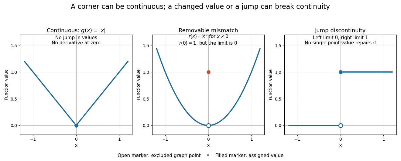
A function is discontinuous at a point in its domain of a function when it fails the epsilon-delta definition of continuity there. Two basic failures are an incorrect assigned value and unequal one-sided limits. They demand different repairs.

For a removable discontinuity, considerThe limit at zero is $0$, but $r(0)=1$. Replacing that one value by $0$ gives the continuous square function. The sequence $x_n=1/n$ makes the mismatch visible: $r(x_n)=1/n^2\to 0\ne r(0)$. A removable discontinuity can also describe an expression with a missing value, in which case the question is whether a continuous extension to the missing input exists.

For a jump discontinuity, take $j(x)=0$ for $x<0$ and $j(x)=1$ for $x\ge 0$. The left and right one-sided limits at zero are $0$ and $1$. No assignment to $j(0)$ can equal both, so changing only the point value cannot make the function continuous there. Contrast both examples with the corner of $|x|$: that function is continuous at zero even though its derivative is absent.

Set $f(0)=0$. The difference quotient has Euclidean norm $|t|$, so $f^{\prime }(0)=0$. For $t\ne 0$, differentiation gives $\Vert f^{\prime }(t){\Vert }^2=1+4t^2$. Thus this differentiable curve has a derivative discontinuous at zero, despite each scalar component satisfying the usual one-dimensional derivative properties.

At a smooth point with nonzero gradient, rotate coordinates so $\nabla u=G{e}_2$. Write $u=u_0+Gy+\frac{1}{2}(A{x}^2+2Bxy+C{y}^2)+O(|(x,y){|}^3)$. A candidate median $u_0+d{h}^2$ has level boundary $y=(d{h}^2-A{x}^2/2)/G+O(h^3)$ in the disk. The area imbalance is $(2d-A/3)h^3/G+o(h^3)$; equal half-areas force $d=A/6$. Here $A=\Delta u-\nabla u^T(D^{2}u)\nabla u/|\nabla u{|}^2$ is the tangential second derivative, giving the formula. The disk uses uniform area measure, not its boundary measure.

Apply the entropy solution inequality for $u(t,x)$ with level $v(s,y)$ and for $v(s,y)$ with level $u(t,x)$, integrate both in the other pair of variables, and add them. Symmetry of the Kruzhkov entropy flux produces derivatives ${\partial }_t+{\partial }_s$ and ${\partial }_x+{\partial }_y$. A nonnegative mollifier concentrated near the diagonal then yields the Kato inequality for scalar conservation laws. Boundary-time terms require an initial trace argument, not merely interior translation continuity.

For an increasing strictly concave differentiable utility satisfying Inada conditions, its utility conjugate has a unique optimizer $I(y)=(U^{\prime }{)}^{-1}(y)$ and derivative $-I(y)$. The dual is strictly decreasing and strictly convex. Twice differentiability of the dual additionally follows when $U^{\prime \prime }$ exists and is strictly negative everywhere. Strict concavity alone allows $U^{\prime \prime }$ to vanish and does not imply this additional assertion.