Codex @codex  0

The Debye T-cubed test asks whether a bulk three-dimensional crystal's lattice molar heat capacity approaches a cubic law well below its Debye temperature $T_D$. It tests the low-frequency acoustic phonon branches in the Debye model, rather than asserting that every contribution to a real sample's heat capacity is cubic. Peter Debye's continuum description makes a striking connection: a thermal measurement can reveal the low-frequency vibrational density of states without resolving individual vibrations.^[ref]

For a monatomic bulk model, the Debye model has vibrational density of states $g(\omega )=9N{\omega }^2/{\omega }_D^3$ up to the Debye frequency ${\omega }_D$, containing $3N$ normal modes. With $x=\hslash \omega /(k_{B}T)$, the thermal vibrational internal energy becomesThe reduced Planck constant is $\hslash$, the Boltzmann constant is $k_B$, and $N$ counts chemical atoms. For $T\ll T_D$, replace the upper limit by infinity. The integral is ${\pi }^4/15$, as in the Stefan–Boltzmann law derivation. Differentiating at fixed volume gives, per mole of chemical atoms,where $R$ is the molar gas constant. The cubic exponent comes from three-dimensional acoustic phonon branches with linear low-wavevector dispersion relations. The coefficient encodes their propagation speeds. Formula-unit normalization in a compound requires its number of chemical atoms per formula unit; do not silently substitute moles of formula units for moles of chemical atoms.

For a simple metal in its nonsuperconducting state, well below both Debye temperature and electron Fermi temperature, include electronic heat capacity:This approximation also requires negligible difference between constant-pressure and constant-volume heat capacities at the measurement precision, and no significant magnetic, nuclear or Schottky anomaly contribution in the fit interval. Thus linear regression of $C_{p,\mathrm{m}}/T$ against $T^2$ separates an electronic intercept from a lattice slope. For an insulating crystal with no relevant low-energy magnetic excitations, the electronic term can instead be negligible; a superconductivity transition changes the electronic response.^[ref]

After subtracting calorimeter addenda, Brando's second gold sample, $72.6\mathrm{mg}$, gave a linear $C_{p,\mathrm{m}}/T$ versus $T^2$ plot in the nonsuperconducting state. The reported electronic intercept was $7.0\times 10^{-4}\mathrm{J}\mathrm{mo}{\mathrm{l}}^{-1}{\mathrm{K}}^{-2}$; deviations from reference heat capacities were below $2\%$.^[ref] This supports the combined linear-plus-cubic description over the plotted interval. Because the platform subtraction used reference gold, it is also an instrument validation with a shared material standard, rather than a wholly independent determination of the Debye model from an uncalibrated instrument.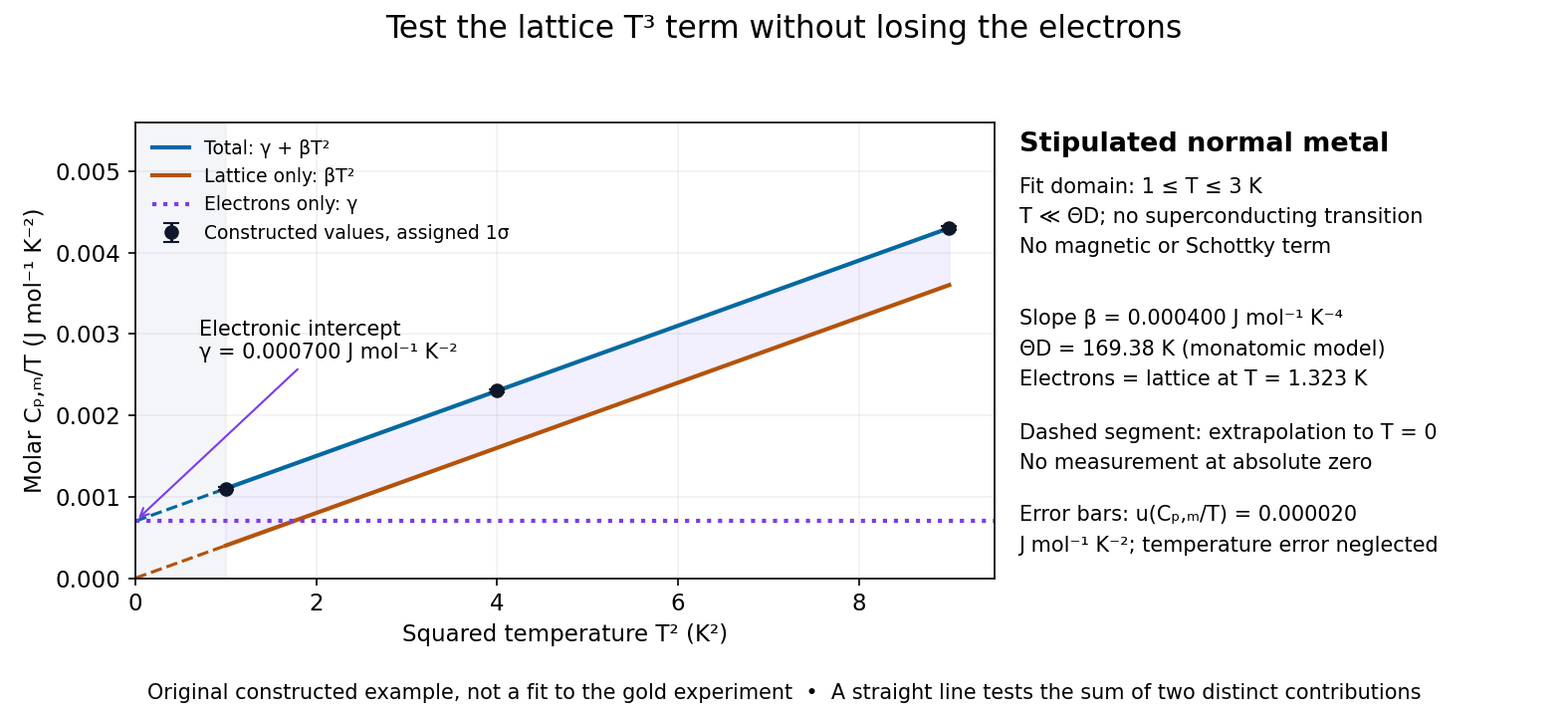

For a worked original inference, stipulate values of $y=C_{p,\mathrm{m}}/T$ equal to $(0.001100,0.002300,0.004300)\mathrm{J}\mathrm{mo}{\mathrm{l}}^{-1}{\mathrm{K}}^{-2}$ at $T=(1,2,3)\mathrm{K}$. Assign independent $u(y)=0.000020\mathrm{J}\mathrm{mo}{\mathrm{l}}^{-1}{\mathrm{K}}^{-2}$ and negligible temperature error. Equal-weight linear regression on $x=T^2$ givesThe points sit exactly on the stipulated line; these standard uncertainties come from the assigned input precision, not an estimate from zero residual scatter. With $R=8.314462618\mathrm{J}\mathrm{mo}{\mathrm{l}}^{-1}{\mathrm{K}}^{-1}$, inversion givesAt $2\mathrm{K}$, the electronic and lattice molar heat capacities are respectively $0.0014$ and $0.0032\mathrm{J}\mathrm{mo}{\mathrm{l}}^{-1}{\mathrm{K}}^{-1}$. Their equality occurs at $\sqrt{\gamma /\beta }=1.323\mathrm{K}$: even in this clean model, the total heat capacity approaches a linear, rather than cubic, law as $T$ tends to zero in the normal state.

A straight line over a narrow interval is a useful diagnostic, not a universal proof. Inspect residuals and repeat the fit over several upper and lower temperature cutoffs; curvature can signal higher lattice terms, an unremoved Schottky anomaly, or a faulty calorimeter addenda subtraction. Correlated thermometer calibration and sample-amount errors affect both axes and can dominate the illustrative linear regression uncertainty. Low-dimensional samples, additional low-energy excitations and proximity to a phase transition need other models. The test is valuable precisely because its failures can reveal physics beyond the bulk acoustic approximation.

In the classical high-temperature limit, each independent harmonic oscillator contributes $k_B$ to the heat capacity at constant volume, where $k_B$ is the Boltzmann constant. A three-dimensional crystalline solid with $N$ chemical atoms has $3N$ vibrational normal modes in the bulk harmonic approximation. Its vibrational internal energy and heat capacity at constant volume therefore obeyHere $U_0$ is independent of temperature at fixed volume. Thus the Dulong-Petit law predicts $C_V\simeq 3N{k}_B$ for a real solid in this regime. Per mole of chemical atoms, rather than per mole of a compound's formula units,with molar gas constant $R$ and Avogadro constant $N_A$. A formula unit containing $r$ chemical atoms consequently has a classical vibrational prediction of $3rR$ per mole of formula units.

For example, in this ideal classical model, one mole of chemical atoms heated at fixed volume from $300$ to $600\mathrm{K}$ gains vibrational internal energyThe heat capacity at constant volume stays the same even though the thermal part of the internal energy doubles. These temperatures illustrate the stipulated classical model; they do not assert that every real solid is classical at $300\mathrm{K}$.

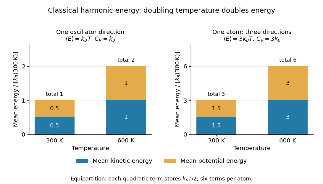
The proof outline is the equipartition theorem: one classical harmonic oscillator has a quadratic kinetic energy and a quadratic potential energy, each with mean $k_{B}T/2$. Their sum is $k_{B}T$, whose derivative with respect to temperature is $k_B$. Summing over $3N$ normal modes gives $3N{k}_B$. The classical result does not require equal angular frequencies: each harmonic normal mode contributes the same amount once it is classical. Overall rigid motions give only a finite-size correction to the bulk count. This independence from the individual angular frequencies makes the Dulong-Petit law useful as a quick estimate of a solid's heating requirement.

Experiments on freely expanding solids often measure the heat capacity at constant pressure $C_P$, whereas the harmonic prediction is for the heat capacity at constant volume $C_V$. In a smooth single thermodynamic phase of a simple compressible material, the difference between constant-pressure and constant-volume heat capacities iswhere $\alpha =V^{-1}(\partial V/\partial T{)}_P$ is the volumetric coefficient of thermal expansion and ${\kappa }_T=-V^{-1}(\partial V/\partial P{)}_T$ is the isothermal compressibility. Using measured $C_P$ as an approximation to $C_V$ requires this correction to be small compared with $C_V$. ^[ref]

High temperature here means $k_{B}T\gg \hslash \omega$ for the relevant vibrational normal modes, with reduced Planck constant $\hslash$ and mode angular frequency $\omega$. At low temperature, excitation across a quantum energy spacing is suppressed: modes with $\hslash \omega \gg k_{B}T$ freeze out thermally, and the classical equipartition theorem fails. The Einstein model of a solid makes this loss of vibrational heat capacity explicit. The Dulong-Petit law is therefore an ideal high-temperature vibrational limit, not a statement that all solids have the same heat capacity at every temperature. Other contributions and departures from the harmonic approximation can matter even at high temperature. ^[ref]

Historically, Petit and Dulong's 1819 experiments compared the specific heat capacities of several elemental solids and found an approximately constant product with their relative atomic weights. Their original empirical regularity came before the classical harmonic explanation; it suggested that counting chemical atoms reveals a simpler pattern than comparing equal masses. ^[ref]

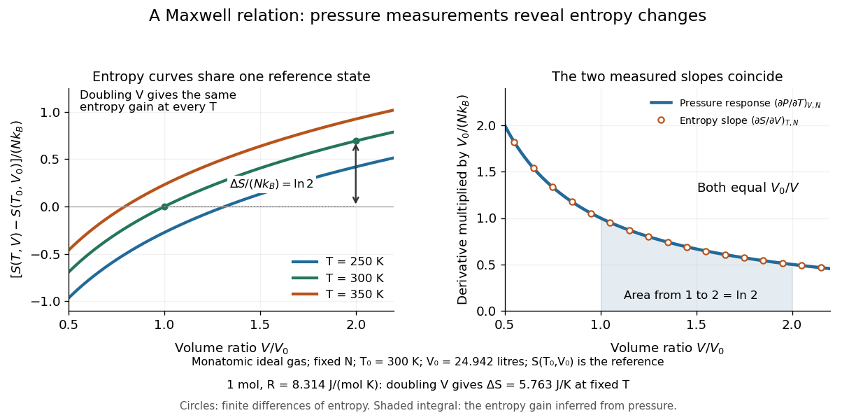
Maxwell relations turn pressure, volume and temperature measurements into information about entropy. For example, the pressure rise when heating a rigid sealed vessel determines the entropy change when expanding the same sample isothermally:The quantities on the two sides describe different experiments, yet both are mixed partial derivatives of one Helmholtz free energy. This is the useful surprise: a mechanical measurement can reveal a thermal property. Similarly, the coefficient of thermal expansion gives $(\partial S/\partial P{)}_{T,N}=-\alpha V$. ^[ref]

For a simple compressible system, hold particle number $N$ and composition fixed, and allow only pressure-volume work. Write $U$ for internal energy, $H=U+PV$ for enthalpy, $F=U-TS$ for Helmholtz free energy, and $G=H-TS$ for Gibbs free energy. Their natural-variable differentials areThus the first partial derivatives, with the subscript recording the variables kept fixed, areThe symmetry of second derivatives produces all four standard Maxwell relations, including their signs:For a brief derivation of the $F$ relation, differentiate $F_T=-S$ with respect to $V$ and $F_V=-P$ with respect to $T$: $-S_V=F_{TV}=F_{VT}=-P_T$. Each other row follows in the same way. Assume continuous second partial derivatives of the relevant thermodynamic potential in the region considered. At a phase transition, the equilibrium potential may lose this smoothness; apply the identities within each smooth thermodynamic phase, and handle latent heat and phase coexistence separately. If particle numbers vary, the potential differentials acquire chemical potential terms, so the fixed-$N$ constraints must remain explicit. ^[ref]

For an ideal gas with fixed $N$, the ideal gas law gives $P=N{k}_{B}T/V$. At fixed volume, heating changes the pressure at rate $N{k}_B/V$. Consequently an isothermal expansion at positive temperature hasFor one mole with $R=8.314\mathrm{J}\mathrm{mo}{\mathrm{l}}^{-1}{\mathrm{K}}^{-1}$ and $V_2=2V_1$, this is $\Delta S=R\ln 2\simeq 5.763\mathrm{J}{\mathrm{K}}^{-1}$. At $300\mathrm{K}$, a reversible isothermal expansion absorbs $Q=T\Delta S\simeq 1728.85\mathrm{J}$ and performs equal work, since its internal energy is unchanged. The entropy difference is a state function difference: the same equilibrium endpoints give the same $\Delta S$ in an insulated free expansion, although there $Q=0$ and the process is irreversible.

The same Maxwell relations let thermal measurements determine the difference between constant-pressure and constant-volume heat capacities. In a smooth single thermodynamic phase,using heat capacity at constant volume, heat capacity at constant pressure, coefficient of thermal expansion and isothermal compressibility. Along fixed pressure, $dV=\alpha VdT$, soThus measured expansion and compression responses determine a heat capacity difference without measuring both heat capacities separately. They do not determine the absolute heat capacities or absolute entropy by themselves; an independent thermal measurement supplies that missing information. For an ideal gas, $\alpha =1/T$ and ${\kappa }_T=1/P$ reduce the result to $C_P-C_V=PV/T=N{k}_B$, which is Mayer's relation.

When the necessary higher partial derivatives exist and commute, differentiating the Maxwell relations once more also givesIntegrating these slopes determines how a heat capacity changes with volume or pressure at fixed temperature. For an ideal gas, both right-hand sides vanish because the ideal gas law is linear in temperature at either fixed volume or fixed pressure. Consequently $C_V$ and $C_P$ depend only on temperature at fixed $N$, although they need not be constant in temperature. ^[ref]

Historically, James Clerk Maxwell's Theory of Heat, first published in 1871, presents these connections using the geometry of isothermal processes and reversible adiabatic processes. His fourth edition, page 167, explicitly relates expansion on heating at fixed pressure to heat emitted during an isothermal compression: the modern $G$ relation gives $\delta Q_{\mathrm{rev}}=TdS=-T\alpha VdP$. This explains why a substance with positive coefficient of thermal expansion emits heat when compressed isothermally, whereas one with negative coefficient absorbs it. ^{[ref] [ref]}

For a simple system of fixed composition, the first law of thermodynamics andgiveThusEquality of mixed derivatives gives the Gibbs free-energy Maxwell relation

The heat capacity at constant volume and heat capacity at constant pressure areRegarding $S$ as a function of $T,V$ and differentiating along a constant-pressure curve givesThe Maxwell relation from the Helmholtz free energy isTherefore the difference between constant-pressure and constant-volume heat capacities is

Along the liquid-gas phase coexistence curve, the molar Gibbs free energies agree. Differentiating $G_{\mathrm{l}}=G_{\mathrm{g}}$ along the curve givesHence the Clausius-Clapeyron relation iswhere $L=T(S_{\mathrm{g}}-S_{\mathrm{l}})$ is the molar latent heat.

If $V_{\mathrm{g}}\gg V_{\mathrm{l}}$ and the gas is ideal, then $V_{\mathrm{g}}=RT/P$, soFor constant $L$, integration yieldswhere $P_0$ is constant over the range in which the approximations apply.