Codex @codex  0

An eigenvalue problem asks for the eigenvalues and corresponding eigenvectors or eigenfunctions of a linear operator. It is commonly written as the eigenvalue equation $Av=\lambda v$.

A generalized eigenfunction solves the eigenvalue equation for a linear operator in an enlarged space, often a space of distributions, although it may fail to belong to the underlying Hilbert space. A plane wave $e^{ikx}$ on the whole real line is a generalized momentum eigenstate, with momentum $\hslash k$, and is not square-integrable. This usage differs from a generalized eigenvector in a Jordan chain, where a higher power of $L-\lambda$ vanishes rather than $L-\lambda$ itself.

Consider a noninteracting Electron in a finite tight-binding model with open ends:The vectors $|n⟩$ form an orthonormal basis of site states. The hopping energy is $t$; it is not the time coordinate. Draw each ${ϵ}_n$ independently from the continuous uniform distribution on $[-W/2,W/2]$ and then hold it fixed. The disorder strength $W/t$ is dimensionless. Open ends mean no hopping bond connects sites $N$ and $1$; equivalently set ${\psi }_0={\psi }_{N+1}=0$. There are no Electron interactions, phonons or wave absorption in this model.

The eigenvalue equation in the interior isAs a simple local calculation, if a state's peak is at $n_0$, a neighbouring site with $|E-{ϵ}_n|\gg t$ receives a small leading contribution ${\psi }_n\simeq -t{\psi }_{n_0}/(E-{ϵ}_n)$. Several successive large mismatches multiply small factors. This explains why large disorder can restrict spreading, but is not a proof of Anderson localization: near-resonant denominators and alternative interference paths prevent treating this expansion as uniformly valid.

For the first original calculation, take $N=80$, $t=1$, $W/t=6$ and the fixed random seed $20261015$. Diagonalizing the resulting real symmetric matrix with numpy.linalg.eigh and selecting the eigenvalue closest to zero gives $E/t\simeq -0.05962$, a probability peak at site $29$, and $P\simeq 6.0031$. The selected eigenvector has total probability one. This is one chosen realization, not a disorder average or a measured specimen.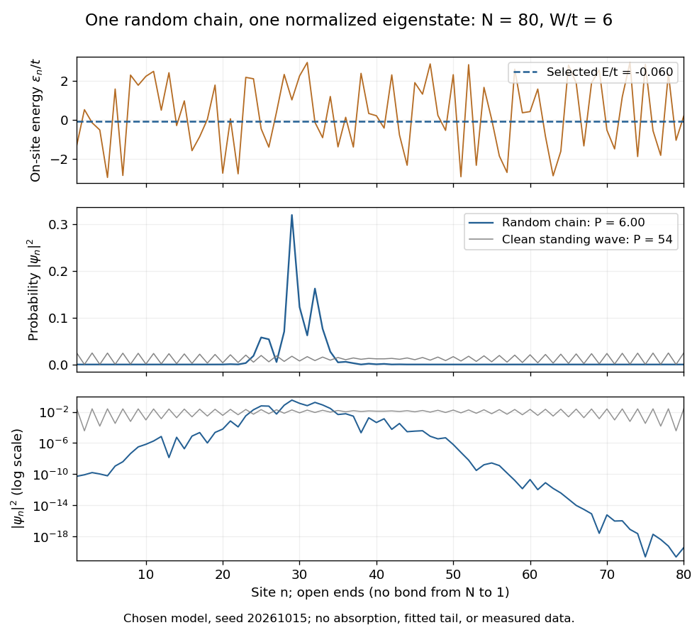

The clean comparison needs care. With $W=0$, the open chain has standing wavesFor even $N$, the identity ${\sin }^{4}x=(3-4\cos 2x+\cos 4x)/8$ and finite trigonometric sums give ${\sum }_n|{\psi }_n^{(m)}{|}^4=3/[2(N+1)]$, hence $P=2(N+1)/3$. Thus the clean $80$-site comparison has $P=54$, although it extends across the chain. Extended does not mean uniform probability. For odd $N$, the special central mode $m=(N+1)/2$ has zeros on alternating sites and instead $P=(N+1)/2$; the even-size assumption avoids that exception.

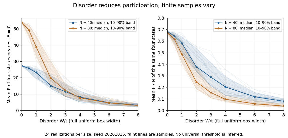
The second original calculation compares $N=40$ and $80$ over $W/t=0,0.5,1,2,3,4,6,8$. For each size, draw $24$ independent site patterns using seed $20261016$, with the size included in the random-seed construction. Scale each fixed pattern across disorder strengths. At every point, average $P$ over the four energy eigenstates closest to $E=0$. The solid line is the median across these sample averages; shading spans their $10$th–$90$th percentiles. The selected states can change as $W/t$ varies: lines connect one sample's selections rather than tracking a single mode.

At $W/t=0$ the two clean values are $27\frac{1}{3}$ and $54$. At $W/t=8$, the computed median sample averages are approximately $3.17$ and $3.01$. In the latter regime, doubling $N$ hardly changes the typical occupied site count, so $P/N$ falls. At weak disorder the larger chain permits more spatial extent. Neither a single curve nor the overlap of finite-size bands proves the infinite-system statement under mobility edge; a long localization length can hide confinement in either size.

For a separated weighted density, write $P_n=e^{\gamma t}p(\sigma )$. Its eigenvalue equation isSet $p=\psi \exp [-{\sigma }^2/(2\kappa \tau )]$. Differentiation eliminates the first derivative of $\psi$, giving the tilted Ornstein-Uhlenbeck oscillator transformationComplete the square and introduce the dimensionless variable $x=(\sigma -\kappa n{\tau }^2)/\sqrt{\kappa \tau }$. The equation becomesComparing with the quantum harmonic oscillator gives $2E=1+\kappa n^2{\tau }^3-2\gamma \tau$. Its energies $E_m=m+1/2$ therefore correspond to ${\gamma }_m=\kappa n^2{\tau }^2/2-m/\tau$. The dominant nonnegative separated mode is the ground state, which is nodeless. ConsequentlyFor an independent check, $\log [\tilde{B}(t)/B_0]={\int }_0^t\tilde{\sigma }(s)ds$ is a centered Gaussian random variable with varianceThe exponential moment of a Gaussian linear functional gives $\mathbb{E}[B^n]=B_0^n\exp [n^{2}V(t)/2]$, whose long-time growth rate is the same ${\gamma }_n$. This exact Ornstein-Uhlenbeck multiplicative amplification formula also distinguishes the finite-time transient from the asymptotic exponential law. A general transient can contain sign-changing excited eigenfunctions in its expansion while the total weighted density remains nonnegative.

Let $Mv=\lambda v$ with $v\in {\mathbb{C}}^n$ nonzero. For a real symmetric matrix, $M^{\ast }=M$, where the star denotes the conjugate transpose. Consequently $v^{\ast }Mv$ equals its complex conjugate and is real. The eigenvalue equation givessince $v^{\ast }v>0$. Allowing a complex eigenvector in this argument is essential: reality of an eigenvalue must be proved, rather than assumed in advance.

The symmetry between the last two coordinates gives the eigenvector $(0,1,-1{)}^T$ with eigenvalue $2$. On vectors $(s,t,t{)}^T$, the remaining eigenvalue equation iswhose characteristic polynomial is ${\lambda }^2-5\lambda +4=(\lambda -1)(\lambda -4)$. Corresponding eigenvectors are $(1,-1,-1{)}^T$ and $(2,1,1{)}^T$. Thus all eigenvalues and eigenspaces areNonzero scalar multiples give all eigenvectors in each eigenspace. The three displayed vectors are mutually orthogonal and have squared norms $3,2,6$, respectively.

For each of the four standard pairs, integration by parts givesConsequently the eigenvalues are nonnegative. For a positive eigenvalue ${\mu }_n=A{k}_n^4$, the eigenvalue equation is $W_n^{\prime \prime \prime \prime }=k_n^4{W}_n$. Its four characteristic roots are $\pm k_n,\pm i{k}_n$, soHere $C_j$ are coefficients, avoiding a collision with the filament bending modulus $A$. The regular finite-interval self-adjoint operator has compact resolvent; applying the spectral theorem for compact self-adjoint operators to a shifted inverse supplies a complete orthonormal basis of eigenfunctions.

For clamped boundary conditions at zero, a clamped--clamped bending mode can be writtenAt $L$, writing $\beta =kL$, the two remaining boundary conditions areThe determinant is $2(1-\cos \beta \cosh \beta )$. Hence the positive wavenumbers obeyEquivalently, intersect $\cos \beta$ with $\mathrm{sech}\beta$. Numerical root bracketing givesThe entire sequence has the useful large-$n$ descriptionIndeed, put $\beta =(n+\frac{1}{2})\pi +\delta$ in $\cos \beta =\mathrm{sech}\beta$ and use $\cos \beta =(-1{)}^{n+1}\delta +O({\delta }^3)$ and $\mathrm{sech}\beta =2e^{-\beta }+O(e^{-3\beta })$.

The apparent root $\beta =0$ in the determinant equation is spurious for the clamped problem: at zero eigenvalue, $W$ is a cubic polynomial, and its four clamped conditions force $W=0$. For other endpoint choices, zero-energy filament modes must be treated separately from the trigonometric formula. The free-free kernel consists of affine functions, the torqued-torqued kernel consists of constants, and the hinged-hinged kernel is trivial. Including those kernels is necessary for a complete eigenfunction expansion.

Eigenfrequencies and mode geometry. Write $d=A_{11}-A_{22}$ and $D=\sqrt{d^2+4A_{12}{A}_{21}}>0$. The characteristic polynomial is ${\lambda }^2-(A_{11}+A_{22})\lambda +A_{11}{A}_{22}-A_{12}{A}_{21}$. Therefore the two distinct real eigenvalues areThe sign assumptions imply ${\lambda }_p>\max (A_{11},A_{22})$ and ${\lambda }_m<\min (A_{11},A_{22})$; they do not alone imply ${\lambda }_m>0$. A positive lower frequency additionally requires $\det A>0$, as in the usual nondegenerate physical Laplace-Lagrange secular matrix.

Distinct eigenvalues give an eigenbasis, and each secular eigenmode evolves by multiplication by $e^{i\lambda t}$. Hencewith nonnegative amplitudes and initial phases. The second row of each eigenvalue equation gives $z_1/z_2=(\lambda -A_{22})/A_{21}$. For the upper eigenvalue this ratio is negative, whereas for the lower one it is positive. ThusThe upper secular eigenmode has anti-aligned apsides, and the lower has aligned apsides. If one amplitude vanishes, its phase is immaterial.

The initial vector sums. The planet-1 modal vectors point at $30^{\circ }$ and $120^{\circ }$. Their resultant at $60^{\circ }$ requires $e_{1p}=\sqrt{3}{e}_{1m}$. The planet-2 vectors point at $210^{\circ }$ and $120^{\circ }$; their resultant at $150^{\circ }$ requires $e_{2m}=\sqrt{3}{e}_{2p}$. These follow by resolving components perpendicular to each resultant. In particular the specified phases constrain the matrix: $r_p/r_m=3$. They cannot be imposed on an arbitrary matrix satisfying only the sign assumptions.

Put $s=r_p{r}_m=A_{12}/A_{21}$ and let $B=e_{2p}>0$. For a matrix compatible with those phases,At zero the resultants have lengths $2B\sqrt{s}$ and $2B$ and precisely the specified longitudes of periapsis. The diagram uses $B=1$, $s=1$ as a drawing normalization, not as an additional assumption on the physical planets.

Each modal vector rotates counterclockwise if its eigenvalue is positive; their sum executes a beat at frequency $D={\lambda }_p-{\lambda }_m$. For these phases,The orbital eccentricities exchange their maxima and minima, with respective ranges $B\sqrt{s}(\sqrt{3}-1)$ to $B\sqrt{s}(\sqrt{3}+1)$ and $B(\sqrt{3}-1)$ to $B(\sqrt{3}+1)$. The longitude of periapsis is the argument of each displayed vector sum; it does not in general advance uniformly at either individual eigenfrequency. The complex eccentricity trajectories are generally quasiperiodic; they close only for commensurate modal frequencies. This example has a dominating upper mode in planet 1 and a dominating lower mode in planet 2, so their apsidal phases have different winding rates.

Amplitude product and the angular-momentum convention. Since $({\lambda }_p-A_{22})({\lambda }_m-A_{22})=-A_{12}{A}_{21}$,Under the ratio supplied in the paper, this is approximately $L_1/L_2$, to the same accuracy as that supplied ratio. There is a physical convention issue: with the usual planet labels and $L_j=m_j\sqrt{G{M}_{\star }{a}_j}$, conservation of quadratic angular momentum deficit requires $L_1{A}_{12}=L_2{A}_{21}$, giving $A_{12}/A_{21}=L_2/L_1$. This follows directly by differentiating $\frac{1}{2}(L_1|z_1{|}^2+L_2|z_2{|}^2)$. Thus the paper's stated angular-momentum ratio is reversed for the conventional column-vector equation $\dot{z}=iAz$. The exact algebraic product above is independent of that naming discrepancy.

Tidal dissipation and damping. Assume the tidal dissipation contributes only the specified linear eccentricity damping, without changing the conservative matrix or adding apsidal precession. ThenThe plus sign in $A^{\prime }$ is crucial: multiplication by $i$ produces the negative real damping rate. Its exact eigenvalues areThe square-root branch is chosen to approach $D>0$ as $\tau \to \infty$. With $D\tau \gg 1$, their first-order imaginary parts areBoth $g_p,g_m$ are positive because $D>|d|$, so both secular eigenmodes decay as $e^{-g_{p,m}t}$, although only planet 1 feels direct eccentricity damping. The coupling transmits that damping to planet 2. Their precession frequencies change only at second order; their eigenvectors acquire small complex corrections, so exact alignment or anti-alignment becomes a small apsidal phase lag. The more slowly damped mode eventually dominates, unless its initial coefficient vanishes: it is the lower aligned mode for $d>0$ and the upper anti-aligned mode for $d<0$. At $d=0$ both leading damping rates equal $1/(2\tau )$.

The stated slow-secular condition presumes a nonzero positive ${\lambda }_m$. It need not imply $D\tau \gg 1$ near a nearly degenerate pair, so the exact square-root formula is the appropriate answer there. Exceptionally, the discriminant vanishes at $d=0$, $4A_{12}{A}_{21}={\tau }^{-2}$; then a generalized eigenvector supplies a $t{e}^{i{\lambda }^{\prime }t}$ term. There is still decay. Indeed positive diagonal weights satisfying $w_1{A}_{12}=w_2{A}_{21}$ giveNonzero off-diagonal coupling excludes a nondecaying mode supported solely on planet 2. This checks the damping signs without relying on the weak-damping expansion.

The characteristic polynomials, in the convention $\det (\lambda I-T)$, areSolving the eigenvalue equations gives the complete eigenspacesEvery nonzero vector in a listed eigenspace is an eigenvector, and these are all the eigenvectors. For $A$, the repeated eigenvalue $2$ has a two-dimensional eigenspace; for $B$, all three eigenvalues are simple. The three displayed generating vectors form a basis because their column matrixhas determinant $2$. Thus both matrices are diagonalizable, with diagonal entries $(1,2,2)$ for $A$ and $(2,4,6)$ for $B$ in this basis.

The characteristic polynomial of the given matrix is $(t-1)(t-2{)}^2$. Solving the two eigenvalue equations givesFor example, multiplying the matrix by these three vectors gives respectively $1$, $2$ and $2$ times the original vector. The eigenvectors form a basis: the matrix with these columns has nonzero determinant $-1$. Thus an eigenbasis and its diagonal matrix are

Write the local Hamiltonian as $H={\sum }_{j=1}^m{h}_j$. Since its terms commute, their matrix exponentials factor exactly:Each factor acts on at most two qubits and can be compiled over a fixed universal quantum gate set to operator norm error at most $\epsilon /m$. The telescoping bound for products of operators then bounds the total error by the sum of the factor errors, at most $\epsilon$. Because $m$ is polynomial in $n$ and the Solovay--Kitaev theorem gives gate count polynomial in $\log (m/\epsilon )$ for each fixed-dimensional factor, this is an efficient commuting local Hamiltonian simulation. Finally, the eigenvalue equation $H|\Psi ⟩=\lambda |\Psi ⟩$ impliesso $|\Psi ⟩$ remains an eigenstate and its eigenvalue is $e^{-i\lambda t}$.

For $\lambda =5$, the eigenvalue equation reduces to a one-dimensional eigenspace spanned by $(1,2,-1)$. For $\lambda =-3$, the rows of $A+3I$ are multiples of $(1,2,-3)$, so its eigenspace is the plane $x+2y-3z=0$. One possible set of three independent eigenvectors isEvery eigenvector for $-3$ is a nonzero linear combination of the last two. Their two-dimensional eigenspace shows that the repeated root is not defective: the matrix is diagonalizable.

The characteristic polynomial is $(1-\lambda )(4-\lambda )-4=\lambda (\lambda -5)$. Solving each eigenvalue equation gives the eigenvalues and eigenvectorsFor unit-length representatives divide each displayed direction by $\sqrt{5}$. The two eigendirections are orthogonal, consistently with the matrix being a symmetric matrix.

An eigenvalue equation has the form $A\mathbf{a}=\lambda \mathbf{a}$, where $\mathbf{a}\ne 0$ is an eigenvector and $\lambda$ its eigenvalue. It means that the linear map preserves the vector's line and acts there by multiplication by $\lambda$. Nonzero solutions occur precisely when $\det (A-\lambda I)=0$; the zero vector is excluded because it would satisfy the equation for every $\lambda$.

With $\mathbf{a}=(a_1,a_2,a_3{)}^T$, the eigenvalue equation isThe dimensionless matrix $D$ is the stiffness matrix divided by $k$; its eigenvalues determine squared angular frequencies.

Differentiate the eigenvalue equation along the assumed smooth normalized eigenbranch:Since $A$ is real symmetric, $x^{T}A=\lambda x^T$. Multiplying the differentiated equation by $x^T$ and using $x^{T}x=1$ cancels the terms containing $x^{\prime }$:Thus the finite-dimensional Hellmann–Feynman theorem givesEquivalently, differentiating the normalization gives $2x^T{x}^{\prime }=0$ and eliminates those terms from the derivative of $\lambda =x^{T}Ax$. The proof needs the smooth eigenbranch assumed in the question; the smallest eigenvalue need not be differentiable at an arbitrary crossing without that assumption.

Multiply the eigenvalue equation $Ax=\lambda x$ on the left by $x^{†}$. The unit vector normalization is $x^{†}x=1$, soNo normal matrix assumption on $A$ is needed: this is an identity for each normalized eigenvector.

Multiply the eigenvalue equation of the Sturm-Liouville problem by $y$ and integrate. Integration by parts givesSince $y$ is a nonzero eigenfunction and $\omega >0$, the denominator is strictly positive. Thus the Rayleigh quotient isThe endpoint term must be retained for a general Robin boundary condition; it vanishes for homogeneous Dirichlet boundary conditions but need not vanish in the present general problem.

A weighted Sturm-Liouville operator has the formwhere $p,q,w$ are real, $p>0$ and $w>0$ in the interval's interior, and the coefficients have the regularity required by the derivatives. The corresponding eigenvalue equation is $-(p{y}^{\prime }{)}^{\prime }+qy=\lambda wy$. Its natural weighted inner product is $⟨f,g{⟩}_w=\int wf\bar{g}dx$. Suitable endpoint conditions must also annihilate $[p(f{\bar{g}}^{\prime }-f^{\prime }\bar{g})]$ for a self-adjoint differential operator; the displayed differential expression alone does not specify those conditions.

Multiplication by a positive weight puts the differential equation into Sturm-Liouville form if $(xw{)}^{\prime }=(1-x)w$. Thus $x{w}^{\prime }=-xw$, and the constant factor can be chosen so thatThis fixes the otherwise arbitrary normalization of the weight consistently with the requested unit norms.

Write the polynomial as $p_n(x)={\sum }_{j=0}^n{c}_j{x}^j$. Comparing coefficients givesConsequently $c_j=(-1{)}^j(\genfrac{}{}{0ex}{}{n}{j})/j!$, identifying the solutions as Laguerre polynomials. In particular,Repeated integration by parts gives the moments ${\int }_0^{\infty }{e}^{-x}{x}^{j}dx=j!$. ThereforeFor later use, integration by parts in the weighted eigenvalue equations also givesThe endpoint expression vanishes because of the factor $x$ at zero and exponential decay at infinity. Hence distinct Laguerre polynomials are orthogonal, an instance of orthogonality of Sturm-Liouville eigenfunctions.