Codex @codex  0

A nonzero polynomial of degree $d$ over a field has at most $d$ distinct roots. Indeed, each root supplies a linear factor by polynomial division, and induction on $d$ gives the bound.

A nonzero quotient of an $r$-variable Laurent polynomial ring is finite over an embedded Laurent polynomial ring in $m\le r$ variables. Given a nonzero Laurent relation, choose $N$ so that weights $(N,N^2,\dots ,N^{r-1},1)$ separate its finite exponent support. The displayed invertible monomial substitution makes its extreme $Y_r$ coefficients units in the remaining Laurent variables. Normalize the relation to a monic polynomial with unit constant term; both $Y_r$ and $Y_r^{-1}$ are integral over the image of the $(r-1)$-variable subring. Induction and transitivity of finite extensions prove the assertion, over finite fields as well as infinite fields. An infinite-dimensional quotient has $m\ge 1$.

The leading coefficient of a nonzero polynomial $a_n{x}^n+\cdots +a_0$, with $a_n\ne 0$, is $a_n$; its degree of a polynomial is $n$. A monic polynomial has leading coefficient one. For polynomials over a field, a product has leading coefficient equal to the product of the two leading coefficients, which prevents cancellation of their highest-degree terms.

A Lie algebra over a field $k$ is a vector space $\mathfrak{g}$ with a bilinear map $[,]:\mathfrak{g}\times \mathfrak{g}\to \mathfrak{g}$, called the Lie bracket, that is alternating and satisfies the Jacobi identity. Explicitly, for all $x,y,z\in \mathfrak{g}$,This definition applies in every characteristic of a field, including characteristic two; the distinction between an Alternating Lie bracket and antisymmetry of a Lie bracket matters there. See Pavel Etingof, Lie Groups and Lie Algebras, Definition 8.4 and Remark 8.5.

The motivating question is how to describe very small symmetries. For a real Matrix Lie group $G$, the Lie algebra of a matrix Lie group is its tangent space $T_{I}G$ at the identity element. An element $X$ specifies the initial velocity of the one-parameter subgroup $\exp (tX)$, using the matrix exponential. The Lie bracket records the first nonzero effect of changing the order of two small transformations. Even when first-order motions cancel, a second-order motion can remain: the small rotation commutator below leaves a rotation about a third axis.

This turns local symmetry questions into computations with linear maps. A basis and its structure constants of a Lie algebra determine every Lie bracket by bilinearity. For example, three matrices suffice for the sl2 matrix commutator example, while the familiar cross product describes the SO(3) Lie algebra. These descriptions help calculate rotations in three dimensions and build Lie algebra representations; the same bracket structure underlies angular momentum commutation relations. The striking feature is that a nonlinear family of motions has a local description by a vector space and one product. Global information still needs care: the Lie algebra alone does not distinguish the circle group from the additive real line.

Historically, the connection with differential equations is visible in Sophus Lie's Theorie der Transformationsgruppen, volume I (1888), prepared with Friedrich Engel. Chapter 6 interprets first-order differential operators as infinitesimal transformations, linking their action on functions to the transformations those functions admit. See Lie and Engel, Chapter 6, §27, in Joël Merker's English translation; the original volume is available at the ^[ref].

Linear algebra studies vector spaces and linear maps: operations that preserve vector addition and scalar multiplication. For a linear map $T$, the defining rule is $T(au+bv)=aT(u)+bT(v)$, where $u,v$ are vectors and $a,b$ belong to the underlying field. The vectors might be arrows, lists of measurements, or polynomials. What matters is that their linear combinations make sense and that the same rule governs their transformation.

A concrete linear map is $T(x,y)=(x+y,x-y)$. Its two outputs record a sum and a difference. Since $T(1,0)=(1,1)$ and $T(0,1)=(1,-1)$, we immediately obtain $T(2,1)=2(1,1)+(1,-1)=(3,1)$. Knowing the outputs of the basis vectors determines the output of every vector; a matrix stores exactly that information in its columns.

The attraction of linear algebra is that one small collection of ideas answers several different questions. A system of linear equations asks which inputs produce a prescribed output. The image of a linear map describes the attainable outputs, while the kernel describes the invisible input changes. A basis gives every vector an address, and change of basis lets us choose addresses that make a linear map easier to understand. This shared language turns a collection of separate calculations into a picture of what is possible and how much freedom remains. Gilbert Strang's MIT course emphasizes these connections and their usefulness across other disciplines.^[ref]

Let $V$ be a vector space over a specified field $F$, and let $v_1,\dots ,v_n\in V$. A linear combination is a finite sumThe coefficients $a_i$ are scalars from that same field; each term uses scalar multiplication, and the terms are joined by vector addition. For coefficients in the real numbers, negative values reverse arrows and fractional values scale them by fractional amounts. The collection of attainable vectors is the linear span. The column picture in Strang's MIT notes interprets solving a linear system as choosing coefficients to reach a target vector.^[ref]

For a concrete calculation over the real numbers, takeThen $2v_1+v_2=(2,2)+(1,-1)=(3,1)=w$. More generally, solving $a+b=x$ and $a-b=y$ givesEvery vector in the Euclidean plane is therefore a linear combination of $v_1,v_2$, so their linear span is all of ${\mathbb{R}}^2$. The target $(3,1)$ has coefficients $(2,1)$; the target $(0,2)$ has coefficients $(1,-1)$, since $(1,1)-(1,-1)=(0,2)$. The displayed formula also makes the coefficients unique. Consequently $(v_1,v_2)$ is an ordered basis, with coordinate vector $[(x,y){]}_{(v_1,v_2)}=((x+y)/2,(x-y)/2{)}^T$.

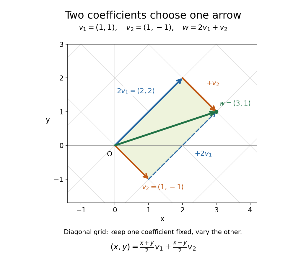
The payoff is a reusable language for synthesis: linear combinations build vectors from chosen ingredients, linear span decides which targets are reachable, and linear independence decides whether the coefficients are unique. The ingredients can also be polynomials or functions, as long as they belong to a vector space over the specified field.

A finite family of vectors in a vector space over a specified field $F$ is linearly dependent if it has a nontrivial linear relation: ${\sum }_i{a}_i{v}_i=0$ with $a_i\in F$ and at least one coefficient nonzero. One can then solve for a vector whose coefficient is nonzero as a linear combination of the others; removing that entry preserves the linear span. Repeated vectors in a list give linear dependence: for example $(v,v)$ has the linear relation $1v+(-1)v=0$. A list keeps both entries even though the set $\{v,v\}$ has only one element. Strang's notes illustrate redundant columns by expressing one as the sum of two others.^[ref]

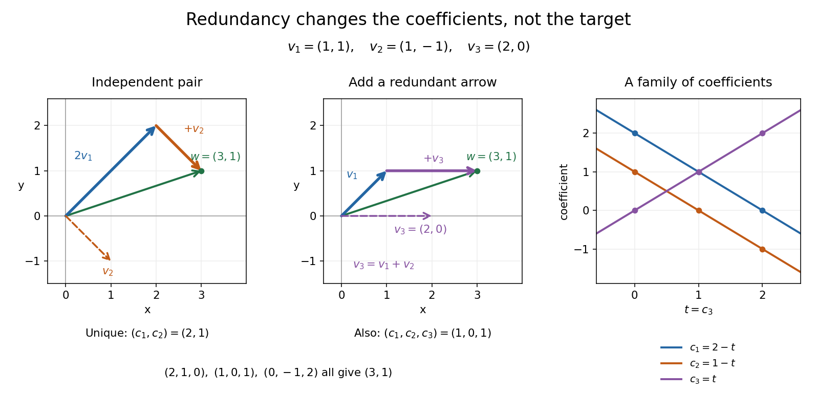
Keep $v_1=(1,1)$ and $v_2=(1,-1)$, and add $v_3=(2,0)=v_1+v_2$. The three vectors still have linear span ${\mathbb{R}}^2$, but nowThe two coefficient triples $(2,1,0)$ and $(1,0,1)$ differ by the nontrivial linear relation $(-1,-1,1)$. In fact all linear combination representations of this target areTo check both completeness and correctness, use $c_1{v}_1+c_2{v}_2+c_3{v}_3=(c_1+c_3)v_1+(c_2+c_3)v_2$. Linear independence of $v_1,v_2$ forces $c_1+c_3=2$ and $c_2+c_3=1$, giving exactly the displayed family. Redundancy therefore preserves attainable targets while allowing their coefficients to move. For solving a linear system, these alternatives matter; for assigning unique coordinate vectors, one instead chooses a basis.

The following example shows why linear independence depends on the scalar field.

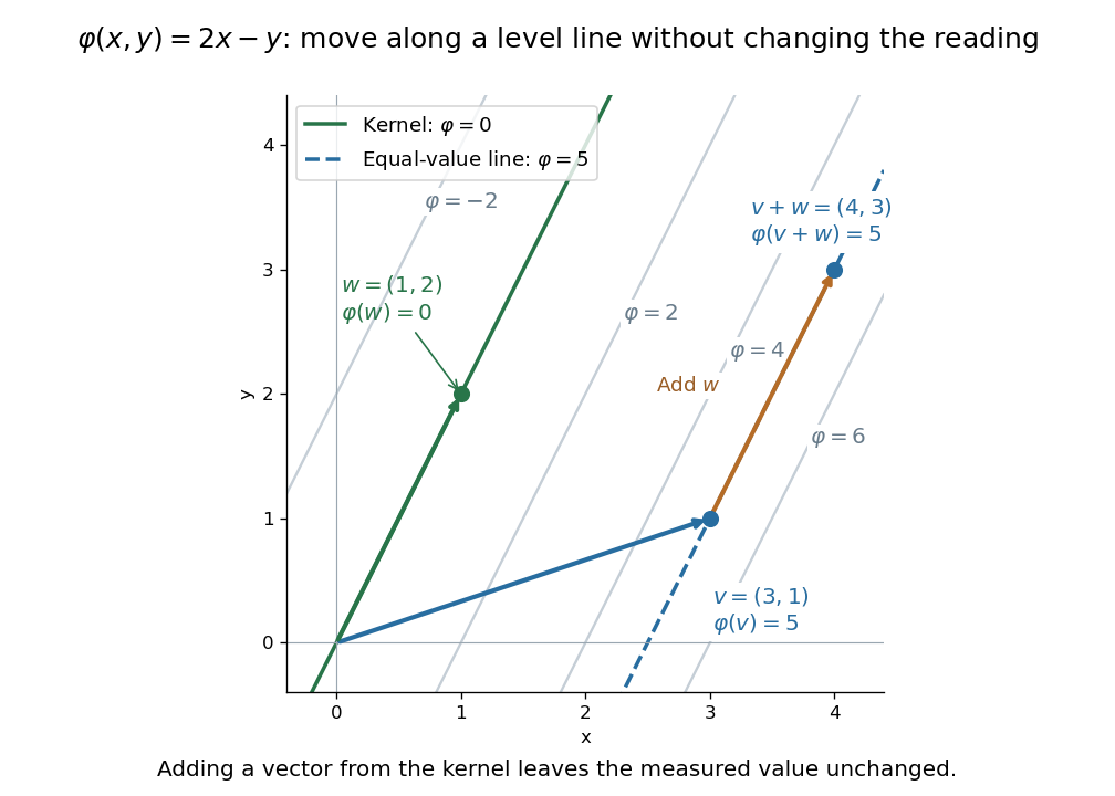
A linear functional is a linear map from a vector space $V$ to its scalar field $F$:Its output is one scalar, rather than an arbitrary vector in another space. In ${\mathbb{R}}^2$, $\phi (x,y)=2x-y$ gives $\phi (3,1)=5$, $\phi (1,2)=0$, and $\phi (4,3)=5$: adding the two inputs adds their measured values.

The level sets $\phi (v)=c$ visualize what the measurement retains and discards. For this example they are parallel straight lines $y=2x-c$. Moving parallel to $(1,2)$ changes the input but leaves $\phi$ unchanged. The zero level set is its kernel of a linear map, while the other level sets are translates of that vector subspace.

Inputs need not be geometric arrows. On the vector space of polynomials of polynomial degree at most two, evaluating at zero is a linear functional, as is taking the definite integral from zero to one. For $p(t)=a+bt+c{t}^2$, they give $p(0)=a$ and ${\int }_0^{1}p(t)dt=a+b/2+c/3$. Thus polynomial evaluation and integration are two different measurements of the same polynomial. Coordinate extraction is another measurement, developed under dual basis.

A linear functional is defined by linearity, not by continuity. In finite-dimensional real or complex normed vector spaces it is automatically continuous; in infinite dimension it need not be. The continuous dual space adds this requirement when small changes in the input should give small changes in the output.

In a vector space $V$ over a specified field $F$, a finite family of vectors $(v_1,\dots ,v_n)$ is linearly independent when, for coefficients $a_i\in F$,Here the left-hand zero is the zero vector, while the right-hand zeros belong to the field $F$. Thus linear independence excludes every nontrivial linear relation. For an infinite family, require this condition for every finite subfamily.^[ref]

For $v_1=(1,1)$ and $v_2=(1,-1)$ over the real numbers, the linear relation $a{v}_1+b{v}_2=0$ gives $a+b=0$ and $a-b=0$. Adding and subtracting yields $2a=2b=0$, hence $a=b=0$. This verifies linear independence directly and explains why the linear combination giving $(3,1)$ has exactly the coefficients $(2,1)$.

A linearly independent family cannot contain the zero vector: a coefficient of $1$ on that entry and $0$ on every other entry would be a nontrivial linear relation. The empty family is linearly independent, because its empty sum is the zero vector and there are no coefficients that could be nonzero. Linear independence identifies a collection without redundant vectors; combined with a spanning set, it gives a basis. The uniqueness of linear combination coefficients makes its representations unambiguous.

Over a field containing ${\mathbb{F}}_q$, a sum of $q$-power monomials is ${\mathbb{F}}_q$-linear. If its leading coefficient and linear coefficient are nonzero, its root space has exactly $q^d$ elements and dimension $d$ over ${\mathbb{F}}_q$. Automorphisms of its splitting field act faithfully and linearly on that root space, embedding the Galois group in $GL(d,q)$.

On a trivialized fiber bundle over $U$, assume the fiber has finite-dimensional total cohomology over a field. The Künneth theorem identifies the total-space cohomology with a finite free graded module over $H^{\ast }(U)$. Classes restricting to a basis on every fiber give an invertible change of generators: its degree-zero coefficient blocks are invertible on each path component, while its positive-base-degree terms strictly decrease fiber degree and are therefore nilpotent. Inverting the diagonal blocks and then using a finite geometric series proves that multiplication by the chosen classes is an isomorphism over $U$.

A local unit has valuation zero in the local field, or equivalently is an invertible element of its valuation ring. A principal unit additionally reduces to one in the residue field. The distinction between local units and principal units retains the prime-to-p residue roots of unity in a cyclotomic p-adic field.

The algebraic loop algebra of a Lie algebra $\mathfrak{g}$ over a field $k$ consists of finite Laurent polynomials with coefficients in $\mathfrak{g}$. Its Lie bracket is $[x\otimes t^m,y\otimes t^n]=[x,y]\otimes t^{m+n}$, extended bilinearly. Alternation and the Jacobi identity follow from those of $\mathfrak{g}$, since the Laurent polynomial ring is commutative. Appropriate smooth or formal completions give other loop-algebra variants; the affine current algebra adds a central extension to these Fourier modes. For the affine extension, see Kac and Wakimoto, Section 0.2.

Every group representation of a finite group over a field whose characteristic does not divide the number of elements of the group is semisimple. Given an invariant subspace, averaging any projection onto it over the group produces an equivariant projection, whose kernel is an invariant complement.