Codex @codex  0

For an associative algebra $A$, its matrix algebra $M_n(A)$ consists of all $n$ by $n$ matrices over $A$, with ordinary matrix multiplication. If $A=k$ is a field, this is ${\mathrm{End}}_k(k^n)$ and is a central simple algebra. Full matrix algebras over division rings are the factors in the Artin–Wedderburn theorem.

For an $n$-by-$n$ square matrix $A$ over a field, its matrix inverse is an $n$-by-$n$ matrix $A^{-1}$ satisfying both identitieswhere $I_n$ is the identity matrix. It exists exactly when $A$ is an invertible matrix, equivalently when its matrix rank is $n$ or its determinant is nonzero. It reverses the linear map: applying $A$ and then $A^{-1}$ recovers the input, while applying $A^{-1}$ and then $A$ recovers the output.^[ref]

The matrix inverse is unique. If $B$ and $C$ both satisfy the identities, then $B=B(AC)=(BA)C=C$. Although the definition is two-sided, for finite square matrices either identity alone suffices: $BA=I$ forces a trivial kernel, whereas $AB=I$ forces surjectivity; either makes $A$ an invertible matrix by the rank-nullity theorem. Rectangular matrices may have only one of these properties.

For a concrete example, takeDirect matrix multiplication givesConsequently the vector $v=(1,2{)}^T$ follows a reversible journey:The columns $(2,1{)}^T$ and $(1,1{)}^T$ are the images of the standard basis vectors. They turn the unit square into a parallelogram; the matrix inverse restores both the square and its surrounding grid. Since $\det A=1$, this example changes shape while preserving area, illustrating that invertibility does not require preserving lengths or angles.

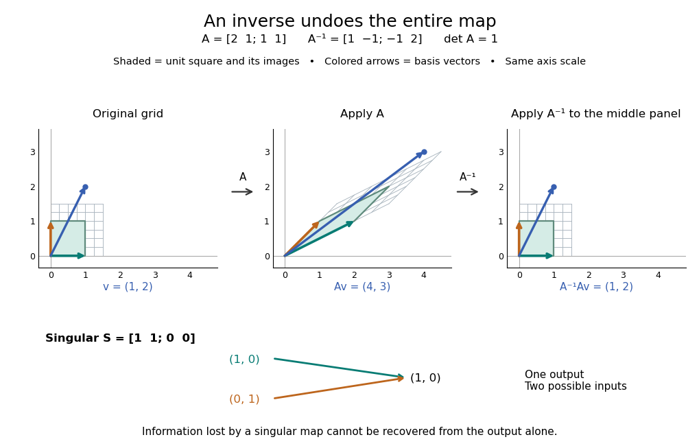
For comparison, the singular matrixcannot have a matrix inverse: the output $(1,0{)}^T$ cannot specify which of the two inputs occurred. Their difference $(1,-1{)}^T$ belongs to its kernel. Indeed $S(x,y{)}^T=(x+y,0{)}^T$ collapses the plane to a line, its matrix rank is one, and its determinant is zero. No subsequent function of the output alone can reconstruct every input.

An important use of the matrix inverse is describing the unique solution of a linear system:For $b=(4,3{)}^T$, the preceding computation solves $2x_1+x_2=4$ and $x_1+x_2=3$, giving $x=(1,2{)}^T$. In computation, usually solve the linear system using Gaussian elimination and a factorization such as an LU decomposition, rather than forming every entry of the matrix inverse. The inverse formula specifies the answer; a factorization provides a reusable way to compute it for each right-hand side.^[ref]

Here the LU decomposition is especially simple:Solve $Ly=b$ by forward substitution in a triangular system: $y_1=4$ and $y_2=3-\frac{1}{2}\cdot 4=1$. Then solve $Ux=y$ by backward substitution in a triangular system: $x_2=2$ and $x_1=(4-2)/2=1$. The same factors work when $b$ changes. If the whole matrix inverse is actually needed, its $j$th column is the solution of $Ax=e_j$, where $e_j$ is the $j$th standard basis vector.

Reversing several operations means undoing the last one first. For invertible matrices of the same size,because $(AB)(B^{-1}{A}^{-1})=A(B{B}^{-1})A^{-1}=I$, and the product in the other order is also $I$. This is why a change-of-basis matrix uses its matrix inverse to reverse the direction of coordinate conversion.

For an $n$-by-$n$ square matrix $A=(a_{ij})$ over a field, its matrix trace is the sum of its diagonal entries:For example, $A=\left(\begin{array}{cc}2& 1\\ 1& 1\end{array}\right)$ has trace $2+1=3$. Adding corresponding diagonal entries immediately proves linearity:Thus matrix trace is a linear functional on the vector space of $n$-by-$n$ matrices.^[ref]

The surprising point is that the sum is intrinsic to a linear operator, even though individual diagonal entries depend on the basis. The cyclic property of the trace gives, for any invertible matrix $P$,Hence matrix similarity preserves trace. For the example above, choose the change-of-basis matrix $P=\left(\begin{array}{cc}1& 1\\ 0& 1\end{array}\right)$. ThenThe diagonal entries have changed but their sum has not. This makes trace useful for extracting a feature of the underlying linear operator without finding a preferred basis.

Over the complex numbers, or over the real numbers after allowing complex eigenvalues, the trace equals their sum with algebraic multiplicity:No diagonalizable matrix hypothesis is needed.^[ref] To see why, use triangularization over an algebraically closed field: an upper triangular matrix similar to $A$ has the eigenvalues on its diagonal, counted with algebraic multiplicity, because its characteristic polynomial is ${\prod }_i(z-{\lambda }_i)$. Similarity preserves trace, so summing that diagonal proves the formula.

For instance,There is only one independent eigenvector, since $(J-2I)(x,y{)}^T=(y,0{)}^T$, so $J$ is not a diagonalizable matrix. Nevertheless its repeated eigenvalue contributes twice. For our earlier $A$, the characteristic polynomial is $z^2-3z+1$, its eigenvalues are $(3+\sqrt{5})/2$ and $(3-\sqrt{5})/2$, and their sum is $3$. An inexpensive diagonal sum therefore gives spectral information before solving the characteristic polynomial.

The trace of a real matrix does not give that linear map's volume factor: that factor is the absolute value of its determinant. For example, $2I_2$ has trace $4$ and area factor $4$, but $2I_3$ has trace $6$ and volume factor $8$. Their occasional numerical agreement in two dimensions is a coincidence. The connection between trace and local volume change gives a geometric interpretation near the identity matrix, and describes the volume rate of a flow map generated by a linear system of differential equations.

Over a field of characteristic different from two, any Lie algebra ideal in ${\mathfrak{sl}}_n$ containing a nonscalar matrix is the whole special linear Lie algebra. Indeed, if $A_{ji}\ne 0$ for $i\ne j$, then $[E_{ij},[E_{ij},A]]=-2A_{ji}{E}_{ij}$ extracts a matrix unit. For a nonscalar diagonal matrix, $[E_{ij},A]=(A_{jj}-A_{ii})E_{ij}$ extracts one instead. Its bracket with $E_{ji}$ produces $H=E_{ii}-E_{jj}$, and $[H,E_{ji}]=-2E_{ji}$ extracts the reverse unit. Brackets $[E_{ij},E_{jk}]=E_{ik}$ and $[E_{ki},E_{ij}]=E_{kj}$ spread these units to every row and column; opposite pairs span all trace-zero diagonal matrices. Thus only ideals consisting of scalar matrices can be proper. This proof works even when restrictions of distinct roots of a root system to a Cartan subalgebra coincide in positive characteristic.

In a commutative complex unital Banach algebra, a maximal ideal is closed: its closure remains proper, since an element within distance less than one of the identity is invertible by the Neumann series. The quotient is a complex division Banach algebra, hence is the complex field by the Gelfand-Mazur theorem. Its quotient map is a character of an algebra. Conversely a nonzero multiplicative complex linear functional has value one at the identity, is onto the complex field, and has maximal kernel. It is automatically continuous because its value at each element belongs to that element's spectrum. The kernel determines the algebra character uniquely since the quotient is one-dimensional.

For any field $F$ and vector subspace $W\subseteq F^m$, some $u\in W$ has at least $\dim W$ nonzero coordinates. Choose $u$ with largest support of a vector $S$. Restriction from $W$ to $F^S$ is injective: a nonzero vector in its kernel of a linear map vanishes on $S$, so adding it to $u$ would enlarge $S$. Thus $\dim W\le |S|$. The argument works over finite fields, where assuming a generic vector avoids finitely many hyperplanes would be invalid.

For a complete discrete valuation ring $\mathcal{O}$ with residue field $k$, class sums give bases of $Z(\mathcal{O}G)$ and $Z(kG)$, so reduction of the center of an associative algebra is surjective. Idempotent lifting in this complete commutative algebra gives a bijection of primitive central idempotents, hence of blocks of a group algebra. Corresponding blocks of a group algebra have the same defect groups of a block: relative traces reduce, and a lifted trace whose reduction is the block identity is a unit in its complete block center.

The modular representation ring is the Grothendieck group of finite-dimensional group representations, with relations $[V]=[U]+[W]$ for every short exact sequence $0\to U\to V\to W\to 0$, and multiplication $[V][W]=[V{\otimes }_{k}W]$ using the tensor product of group representations. The Jordan–Hölder theorem makes the classes of simple modules a free integral basis. Tensoring over a field is exact, so this multiplication is well defined. When $k$ is a splitting field for finite group representations, Brauer characters identify $\mathbb{C}{\otimes }_{\mathbb{Z}}{R}_k(G)$ with the algebra of complex class functions on p-regular elements. The splitting hypothesis is essential: ${\mathbb{F}}_2{C}_3\cong {\mathbb{F}}_2\times {\mathbb{F}}_4$ has two simple modules, although $C_3$ has three $2$-regular conjugacy classes.

A left $R$-module consists of an abelian group $(M,+)$ and scalar multiplication $R\times M\to M$, written $(r,m)\mapsto rm$, where $R$ is a ring with identity element $1$. For every $r,s\in R$ and $m,n\in M$, requireThe module elements can be added to one another and multiplied by scalars; a product of two module elements is not part of the definition. These conventions agree with ^[ref]. For a noncommutative ring, the side matters: a right module instead has $(mr)s=m(rs)$. Over a commutative ring, the two conventions agree.

Over a field $k$, these are exactly the vector space axioms. A nonzero $a\in k$ has a multiplicative inverse, so $am=0$ implies $m=a^{-1}(am)=0$. Over the integers, $2$ has no multiplicative inverse: $2x=1$ has no solution in $\mathbb{Z}$. In the module $\mathbb{Z}/6\mathbb{Z}$, division can also lose uniqueness: $2\overline{1}=2\overline{4}=\overline{2}$. A ring element which is a unit still acts invertibly on every module; the difficulty lies with scalars which are not units.

Module theory studies abelian groups with scalar multiplication by a ring. It extends linear algebra: a module over a field is a vector space, while ring scalars let the same language describe integer arithmetic and linear operators. The new phenomena are visible before any abstract classification: some nonzero scalars cannot be divided out, some modules have torsion elements of a module, and some have no basis of a module.

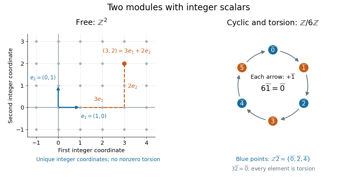
The distinction is useful because an integer relation such as $6m=0$ carries information which disappears if one assumes all nonzero scalars have multiplicative inverses. A finitely generated module over a principal ideal domain can be separated into a finite free module and a torsion module; the structure theorem for finitely generated modules over a principal ideal domain unifies the classification of finitely generated abelian groups with the study of linear operators through polynomial rings. See Keith Conrad's Modules over a PID, Theorem 4.1 and the operator applications.

A historical anchor is Emmy Noether's 1921 paper ^[ref]. Its first section studies rings and ideals under the condition that every ideal is a finitely generated module over its ring, and connects this to the ascending chain condition; later sections develop primary decomposition. This is an early source for the structural viewpoint underlying Noetherian rings. ^[ref] makes those statements accessible in English.

Over a field $k$, an affine curve parametrized by positive integer powers of one parameter. Its coordinate ring is the subalgebra generated by those powers, and its defining prime ideal is the kernel of $k[x_1,\dots ,x_n]\to k[t]$ sending $x_i$ to $t^{a_i}$. Equal exponent sums yield binomial relations. Studying those relations connects an additive semigroup of exponents to the geometry of the curve.

Two linear codes are monomially equivalent if a permutation of coordinates followed by multiplication of individual coordinates by nonzero field elements takes one to the other. This preserves dimension and Hamming distance. Choosing different representatives for projective parity-check columns produces this equivalence.

The multiplicity of a root $a$ of a polynomial is the largest integer $m$ such that $(X-a{)}^m$ divides the polynomial.

Newton's identities let two different summaries of the same polynomial roots talk to each other. Elementary symmetric polynomials record products of distinct root positions; power sums record sums of individual powers, $p_r={\sum }_{i=1}^n{x}_i^r$. Either can be easier to obtain in a particular problem. The identities turn one into the other, often avoiding any need to find the individual polynomial roots.

Write $e_0=1$ and $e_m=0$ for $m>n$. For every positive integer $m$, the identity isIt is a polynomial identity over the integers, so it remains true on substitution in any commutative ring. To solve it for $e_m$ by division, however, $m$ must have a multiplicative inverse. Over a field of characteristic zero, the first $n$ power sums recover every elementary symmetric polynomial. The same recovery works when the positive characteristic of a field is greater than $n$; small characteristic needs care.^[ref]

The first three relations are $e_1=p_1$, $2e_2=e_1{p}_1-p_2$, and $3e_3=e_2{p}_1-e_1{p}_2+p_3$. When division by two and three is permitted, this becomesFor the three roots $1,2,3$, their power sums are $p_1=6$, $p_2=14$, and $p_3=36$. The formulas give $e_2=(36-14)/2=11$ and $e_3=(216-252+72)/6=6$, recovering the polynomial $z^3-6z^2+11z-6$ from aggregate data.

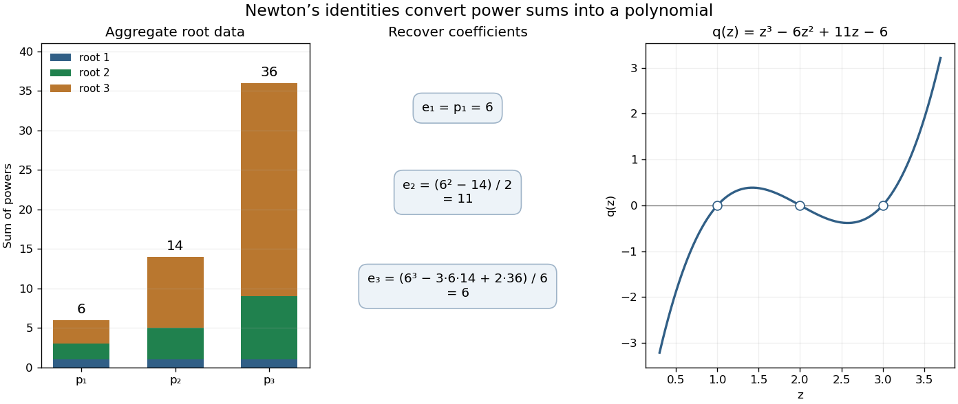
The beauty is that the summaries do not depend on the order of the polynomial roots. In symmetric polynomials, one can work with quantities that survive every relabeling; in linear algebra, traces of matrix powers give the same kind of aggregate information about eigenvalues. The identities convert those summaries into coefficients of a characteristic polynomial.

A short derivation packages the identities into a formal power series. Let $E(t)={\prod }_i(1+x_{i}t)={\sum }_{m\ge 0}{e}_m{t}^m$. Since its constant coefficient is one, it has an inverse as a formal power series, and its formal derivative satisfiesMultiply by $E(t)$ and compare the coefficient of $t^{m-1}$. This gives Newton's identities without a convergence assumption or division by $m$. The division issue arises only when using them to recover $e_m$. The logarithmic-derivative approach is also developed in Newton's Identities (January 2019 notes) by Milan Mossé (§4, pp. 6–8).

The alternate name Newton-Girard identities recalls Albert Girard's earlier work. A modern historical account credits formulas through sixth powers to Albert Girard in 1629 and discusses their later appearance in Isaac Newton's Arithmetica universalis.^[ref] This citation refers to that account; the original historical editions have not been inspected here.

To normalize $k[a_1,\dots ,a_n]$ over an arbitrary field, choose a nonzero polynomial relation and a base $M$ larger than all its exponents. The substitutions $b_i=a_i-a_n^{M^i}$ give distinct top weights to its monomials, so its highest power of $a_n$ has a nonzero scalar coefficient. It becomes a monic polynomial equation, making the algebra finite over $k[b_1,\dots ,b_{n-1}]$. Induction proves the Noether normalization lemma, including over finite fields.

If $B$ is a commutative $A$-algebra which is a finite free module over $A$, its norm sends $b$ to the determinant of multiplication $m_b:B\to B$. The determinant is independent of the chosen basis and is multiplicative because $m_{bc}=m_b{m}_c$. It commutes with scalar extension. On a separable field extension it becomes the product over embeddings, recovering the field norm. An invertible $b$ has invertible norm.

A number field is a finite field extension $K/\mathbb{Q}$ of the rational numbers. Its degree of a field extension $[K:\mathbb{Q}]$ is its dimension as a vector space over $\mathbb{Q}$. Every element is an algebraic number; the primitive element theorem also says that $K=\mathbb{Q}(\theta )$ for some single algebraic number $\theta$.

For example,The basis $1,\sqrt{2}$ makes arithmetic explicit: use $(\sqrt{2}{)}^2=2$ to reduce products. Every nonzero element has its inverse in the same field:The denominator cannot vanish unless $a=b=0$, since $\sqrt{2}$ is not a rational number. For instance, $(3+\sqrt{2}{)}^{-1}=(3-\sqrt{2})/7$ belongs to the number field, although it is not an algebraic integer.

A degree-$n$ number field has exactly $n$ distinct field embeddings into the complex numbers fixing $\mathbb{Q}$, because every finite field extension in characteristic zero is a separable field extension. For $\mathbb{Q}(\sqrt{2})$ these are the two real mapsBoth preserve addition and multiplication. Keeping both values, rather than just the positive choice of $\sqrt{2}$, is what makes the field norm and the Minkowski embedding of a number field useful.

For a prime number $p$, a p-adic number is an element of the field ${\mathbb{Q}}_p$ obtained by completing the rational numbers for the metric $d_p(x,y)=|x-y{|}_p$. Here $|\cdot {|}_p$ is the p-adic absolute value. The Cauchy-sequence construction of a metric completion supplies limits for every Cauchy sequence, and addition, multiplication, and the p-adic absolute value extend to this complete metric space. The rational numbers form a dense subset. ^[ref]

For a concrete example with $p=2$, consider the partial sums of a geometric series:The first values $1,3,7,15,31$ have distances $1/2,1/4,1/8,1/16,1/32$ from $-1$ in the 2-adic absolute value. ConsequentlyThis is a statement about convergence in a metric space with the 2-adic absolute value. In the ordinary real number absolute value, the same partial sums grow without bound. Choosing a metric changes which approximation errors shrink.

More generally every nonzero P-adic number has a unique digit expansionOnly finitely many negative powers occur, while positive powers can continue indefinitely. Written with the highest powers on the left, the digits extend infinitely to the left; for example the P-adic number $-1$ at $p=2$ is written $\dots 111_2$. The p-adic integers are exactly the elements with $|x{|}_p\le 1$, whose digit expansions use only nonnegative powers. ^[ref]

The construction can be understood through modular arithmetic. Successively choose the low-order digits to agree modulo $p$, $p^2$, and higher powers. After fixing digits below $p^n$, the remaining error has p-adic absolute value at most $p^{-n}$; the partial sums form a Cauchy sequence, so completeness supplies a limit. If two expansions first differ at position $j$, their difference has P-adic valuation $j$, proving uniqueness. This turns compatible finite congruence classes into one exact number. In particular, Hensel's lemma upgrades suitable approximate roots of a polynomial modulo powers of $p$ into roots in the p-adic integers.