Codex @codex  0

If $f\in k[Y][X]$ is monic of positive degree in $X$, monic division makes $k[Y][X]/(f)$ free of rank ${\mathrm{deg}}_{X}f$ over $k[Y]$. The inclusion of $k[Y]$ is injective and the quotient is an integral extension, so its Krull dimension is one. This argument applies even when the polynomial factors or the field has positive characteristic.

The dimension of a vector space is the cardinality of any of its bases. In finite dimension this counts the scalars needed to specify an arbitrary vector once an ordered basis is chosen. The exchange argument behind the basis extension theorem shows that any two finite bases have the same size: an independent family cannot be larger than a spanning family.

Thus ${\mathbb{R}}^2$ has dimension two even with an oblique basis, $\mathbb{R}[x{]}_{\le 2}$ has dimension three, and the homogeneous plane in vector subspace has dimension two. This count concerns independent freedom, so an embedded plane remains two-dimensional while sitting in a three-dimensional ambient vector space. Dimension also depends on the field, as the two interpretations of $\mathbb{C}$ in vector space illustrate.

A division algebra over a field $k$ is a division ring equipped with a unital algebra structure over $k$, with $k$ mapping into its center of an associative algebra. Every nonzero element is invertible; it need not be finite-dimensional over $k$.

The ring $k\times k$, for a field $k$, has two prime ideals, $0\times k$ and $k\times 0$. Their localizations at a prime ideal are both isomorphic to $k$. Nevertheless $(1,0)(0,1)=0$ is a product of nonzero elements, so $A$ is not an integral domain. Nonzero orthogonal idempotents separate the two components of its spectrum of a commutative ring.

Let $t$ be a Young tableau of shape $\lambda$, and let $u$ be a Young tableau of shape $\mu$, both on $n$ entries. If the Column antisymmetrizer of a Young tableau $b_t$ satisfies $b_t\{u\}\ne 0$ over any field, then $\lambda$ dominates $\mu$ in the dominance order on partitions.

If two entries from one column of $t$ lie in the same row of $u$, their transposition fixes the tabloid $\{u\}$. Pairing terms of $b_t$ by this transposition gives $b_t\{u\}=0$, including in characteristic two. Otherwise the first $r$ rows of $u$ contain at most $\min (r,{\lambda }_j^{\prime })$ entries from column $j$ of $t$. Thusfor every $r$, proving dominance.

The dual-number ring over a field $k$ consists of elements $a+b\epsilon$ with ${\epsilon }^2=0$. The element $\epsilon$ is a nonzero nilpotent element; its ideal is the ring's only prime ideal. Hence its affine scheme has the same one-point topology as $\mathrm{Spec}k$ while its structure sheaf differs.

The dual space of a vector space $V$ over a field $F$ is the vector space of all linear functionals $\phi :V\to F$. Think of a vector as an input and a linear functional as a scalar-valued measurement of that input. For $V={\mathbb{R}}^2$, the rules $(x,y)\mapsto x$, $(x,y)\mapsto y$, and $(x,y)\mapsto 2x-y$ are different elements of the dual space. None needs a notion of length or angle.

Its operations combine measurements pointwise:The dual basis explains the finite-dimensional structure: specifying a linear functional's values on a basis determines its value on every vector. Thus an $n$-dimensional vector space has an $n$-dimensional dual space. The spaces have the same dimension, but their elements play different roles: an input and a rule that measures an input. ^[ref].

This separation is useful when changing coordinates. The dual pairing $\phi (v)$ must stay the same while the component lists for $v$ and $\phi$ change in opposite ways. Covector transformation under a change of basis makes the compensation explicit. An inner product on a finite-dimensional real vector space gives one way to represent each linear functional by a vector, but that representation uses the chosen inner product; the dual space itself does not require one.

Here dual space means the algebraic dual: all linear functionals. For a topological vector space, the continuous dual space keeps only the continuous linear functionals. In infinite dimension, this can be a proper vector subspace; discontinuous functional detected by vanishing sequence tails gives an example. The distinction matters when a scalar-valued measurement must respond continuously to small input changes.

If $T$ preserves a nondegenerate bilinear form $\omega$ that is alternating and satisfies $T^2=I$ on a finite-dimensional vector space over a field of characteristic different from two, thenThe two eigenspaces are orthogonal for $\omega$, since $\omega (v_{+},v_{-})=\omega (T{v}_{+},T{v}_{-})=-\omega (v_{+},v_{-})$. Each restricted form is nondegenerate: a vector annihilating its own eigenspace also annihilates the other and hence all of $V$. Both dimensions are even, say $2a$ and $2b$. Consequently $\mathrm{tr}T=2a-2b=\dim V-4b$ as an integer obtained from the eigenspace dimensions. Over the real numbers this gives the congruence $\mathrm{tr}T\equiv \dim V(\mathrm{mod}4)$.

A scalar $\lambda$ is an eigenvalue of a linear operator $A:V\to V$ whenfor some nonzero vector $v$, called an eigenvector. The scalar must belong to the field over which $V$ is a vector space. Geometrically, a real eigenvalue tells us what $A$ does along a special line: every vector on that line is multiplied by the same number. The eigenvector gives the line and the eigenvalue gives its scaling.

For a real eigenvalue, $\lambda >0$ preserves the orientation along the line, $\lambda <0$ reverses it, and $\lambda =0$ collapses the line to zero. The length is multiplied by the modulus $|\lambda |$, so $|\lambda |>1$ stretches and $0<|\lambda |<1$ contracts. For example, the diagonal matrix $\mathrm{diag}(2,-1/2,0)$ doubles one coordinate direction, reverses and halves another, and annihilates the third. Its eigenvalues are $2,-1/2,0$; the last direction lies in its kernel.

For a finite square matrix, the eigenvalues are the roots of a polynomial $p_A$, its characteristic polynomial:Here $I$ is the identity matrix. The reason is that $Av=\lambda v$ means $(A-\lambda I)v=0$ with $v\ne 0$: the shifted matrix must have a nontrivial kernel, equivalently a zero determinant. The worked symmetric matrix example in eigenvector shows both stages: find the eigenvalues, then find their eigenspaces.

Eigenvalues are especially useful for repeated application of a linear map. If $Av=\lambda v$, thenOne multiplication proves the next step, so a matrix power becomes an ordinary power on each eigenvector. This explains growth, decay, and alternating signs along these directions. Gilbert Strang develops this connection, and its extension to the matrix exponential, in his lecture "Eigenvalues and Eigenvectors" (MIT 18.065, 2018).^[ref]

A documented historical connection is C. G. J. Jacobi's "Über ein leichtes Verfahren die in der Theorie der Säcularstörungen vorkommenden Gleichungen numerisch aufzulösen" (1846, Journal für die reine und angewandte Mathematik 30, pp. 51–94). Its opening discusses symmetric matrices arising from small oscillations, with a common unknown subtracted from every diagonal entry. In modern notation this is $(A-\lambda I)v=0$; Jacobi seeks the parameter and the ratios of the components of $v$. This is evidence of an early physical and computational setting for the eigenvalue problem, without assigning its discovery to a single person.^[ref][ref]

A nonzero vector $v$ is an eigenvector of a linear operator $A$ when $Av=\lambda v$ for some eigenvalue $\lambda$. For a real vector space and $\lambda \ne 0$, the line through $v$ is preserved: the image can point forward or backward, but cannot turn away from that line. When $\lambda =0$, the image is zero and has no direction. The zero vector is excluded because it satisfies the equation for every scalar and identifies no special direction.

Every nonzero scalar multiple of an eigenvector is an eigenvector for the same eigenvalue, since $A(cv)=cAv=\lambda (cv)$. Thus there is usually no preferred length or sign; choosing a unit vector is a convenient normalization. Eigenvectors for a fixed eigenvalue, together with zero, form its eigenspace.

For a fully computed example, consider the real symmetric matrixIts characteristic polynomial isFor $\lambda =3$, $(A-3I)v=0$ gives $-x+y=0$, so $v_3=(1,1{)}^T$ is an eigenvector. For $\lambda =1$, $(A-I)v=0$ gives $x+y=0$, so $v_1=(1,-1{)}^T$ is an eigenvector. Direct multiplication checks both:The map stretches the line $y=x$ threefold and fixes the line $y=-x$ pointwise. These eigenvectors are orthogonal because $v_3^T{v}_1=0$; dividing each by $\sqrt{2}$ gives an orthonormal basis. A general vector turns because its components along these two lines receive different scalings. For example, $(1,0{)}^T$ maps to $(2,1{)}^T$ and is not an eigenvector.

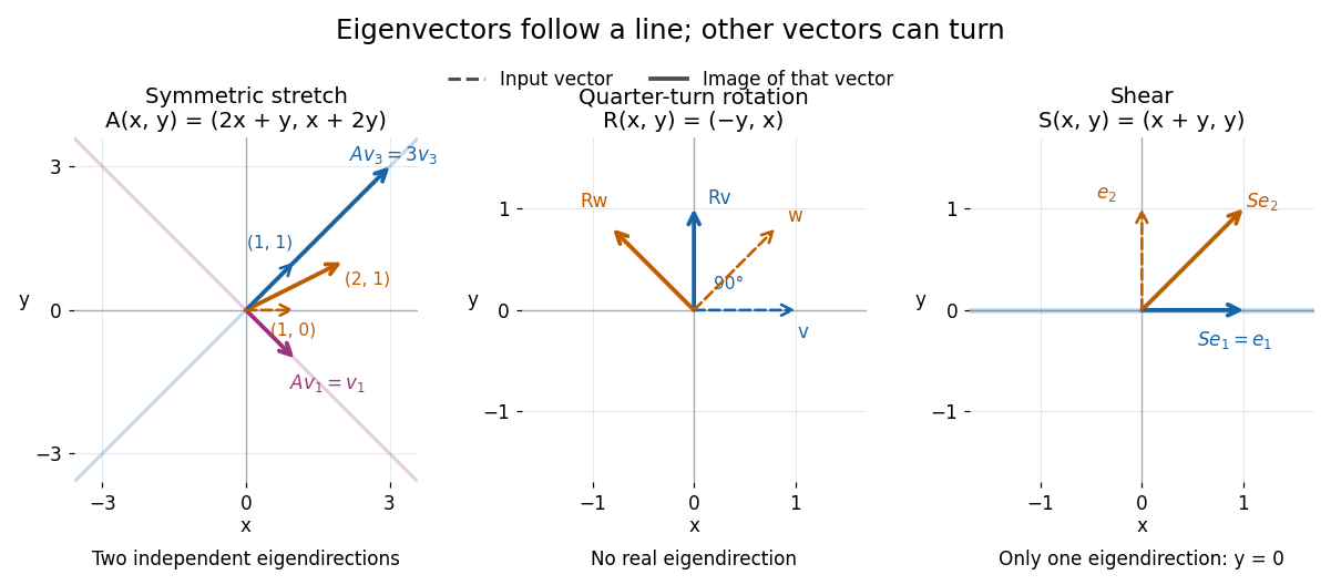
A contrasting example is the planar rotation through $90$ degrees:Every nonzero real vector turns to a perpendicular direction, so there are no real eigenvectors. Its characteristic polynomial is ${\lambda }^2+1$, which has no real roots. Over the complex numbers, however, $R(1,-i{)}^T=i(1,-i{)}^T$ and $R(1,i{)}^T=-i(1,i{)}^T$. The same matrix therefore has an eigenbasis in ${\mathbb{C}}^2$ even though it has none in ${\mathbb{R}}^2$: the choice of field matters.

Two equations are equivalent on a specified domain of a function if they have the same solution set. Adding the same defined mathematical expression to both sides is reversible. Multiplying or dividing both sides by a mathematical expression is reversible only where that expression is nonzero and invertible in the arithmetic being used. In a field, every nonzero scalar is invertible; a general ring needs an additional check.

For example, $x^2=1$ and $(x-1)(x+1)=0$ are equivalent equations over the real numbers, by the distributive property. Concluding $x=1$ or $x=-1$ additionally uses the absence of zero divisors. The modular example in algebra shows why that extra inference can fail in a ring with zero divisors.

For a polynomial $f$ over a field, $f(a)=0$ exactly when $X-a$ divides $f(X)$. Polynomial division gives $f(X)=(X-a)q(X)+f(a)$.

In a field of characteristic $p$, take a basis $e_0,\dots ,e_{p-1}$, and let $x{e}_j=e_{j-1}$ with indices modulo $p$, while $y{e}_j=j{e}_j$. Then $[x,y]=x$, so $kx+ky$ is a solvable Lie algebra, but the distinct eigenvalues of $y$ force any common eigenvector to be a coordinate vector, and $x$ cyclically permutes those vectors. There is consequently no common eigenvector, even over an algebraically closed field.

A field automorphism is a bijective ring homomorphism from a field to itself. The automorphisms fixing a specified subfield form a Galois group when the extension is Galois.

Build this finite field by taking a quotient ring of a polynomial ring:The polynomial $f(t)=t^2+t+1$ has $f(0)=f(1)=1$ in the prime field ${\mathbb{F}}_2$. A polynomial of polynomial degree two is an irreducible polynomial exactly when it has no polynomial root in the coefficient field. Thus the quotient by an irreducible polynomial is a field construction applies. Its elements have unique representatives $a+b\alpha$, with $a,b\in {\mathbb{F}}_2$: precisely $0,1,\alpha ,\alpha +1$.

The defining relation is ${\alpha }^2+\alpha +1=0$. Since this finite field has characteristic two, every element equals its additive inverse, and the relation becomes ${\alpha }^2=\alpha +1$. Addition acts separately on the two coefficients:All coefficient calculations use modular arithmetic modulo two. For example, $(\alpha +1)+\alpha =1$ and $(\alpha +1)+(\alpha +1)=0$. Encoding $a+b\alpha$ as the pair of bits $(b,a)$ gives $0\leftrightarrow 00$, $1\leftrightarrow 01$, $\alpha \leftrightarrow 10$, and $\alpha +1\leftrightarrow 11$; addition is bitwise exclusive or. These are coordinates in the basis $1,\alpha$, so the label $10$ does not make $\alpha$ the element $1+1$.

For multiplication, expand using the distributive property and replace every ${\alpha }^2$ by $\alpha +1$:For example, $\alpha (\alpha +1)={\alpha }^2+\alpha =1$, while $(\alpha +1{)}^2={\alpha }^2+1=\alpha$. The following complete tables are computed from the coefficient rules. Colors identify results, rather than their numerical sizes. Every row of the addition table lists all four elements, and every nonzero row of the multiplication table does too: adding an element, or multiplying by a nonzero element, can be undone.

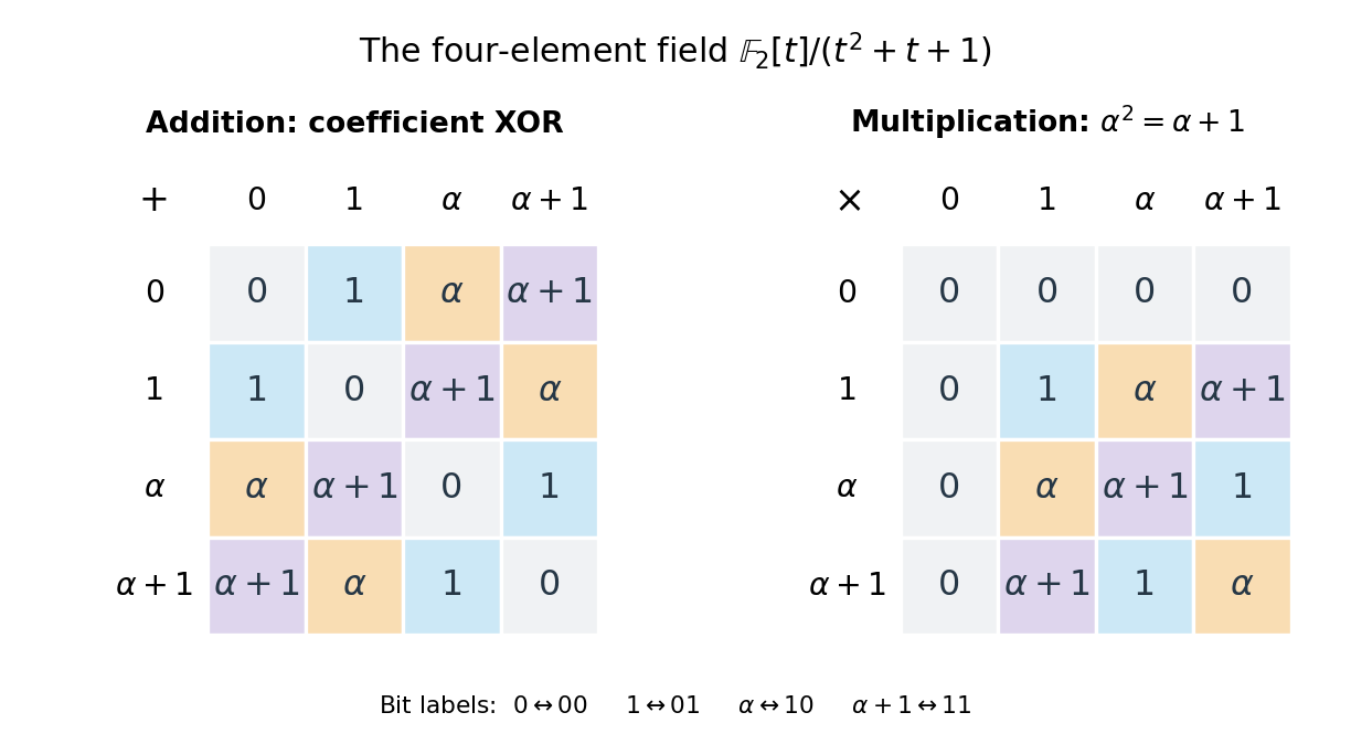
The nonzero multiplicative inverses are $1^{-1}=1$, ${\alpha }^{-1}=\alpha +1$, and $(\alpha +1{)}^{-1}=\alpha$. Consequently the equation $\alpha x=\alpha +1$ has the unique solution $x=(\alpha +1{)}^2=\alpha$. Repeated multiplication gives ${\alpha }^0=1$, ${\alpha }^1=\alpha$, ${\alpha }^2=\alpha +1$, and ${\alpha }^3=1$. They cycle through every element of the multiplicative group of a finite field.

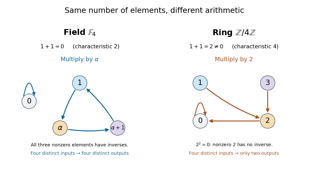
Compare the ring $\mathbb{Z}/4\mathbb{Z}$, also with four elements. Its addition satisfies $1+1=2\ne 0$, and its multiplication satisfies $2^2=0$. Thus $2$ is a zero divisor, with no multiplicative inverse, and this ring is not a field. Multiplying by $2$ collapses different inputs to the same output: both $0$ and $2$ give $0$, while both $1$ and $3$ give $2$. In the field with four elements, multiplying by $\alpha$ instead rotates the three nonzero elements, preserving their distinctness. The figure makes visible why counting four elements alone does not specify their arithmetic.

A finite field is a field with finitely many elements: addition, subtraction, multiplication, and division by a nonzero element all stay inside a finite collection. Write ${\mathbb{F}}_q$, or $\mathrm{GF}(q)$, for a finite field with $q$ elements. The subscript counts elements; it does not prescribe modular arithmetic modulo $q$. The field with four elements is the smallest example where that distinction matters.

Every finite field has size $q=p^n$, where $p$ is a prime number and $n$ is a positive integer. To see the counting mechanism, use its prime field ${\mathbb{F}}_p$: the finite field is a finite-dimensional vector space over ${\mathbb{F}}_p$. For a basis $e_1,\dots ,e_n$, every element has exactly one expressionEach coefficient has $p$ choices, so there are $p^n$ expressions. Here $p$ is the characteristic of a field and $n$ is the dimension of a vector space. Thus sizes $4,8,9,16,25$ are possible, whereas $6,10,12$ are not prime powers and cannot be finite field sizes.

Conversely, every prime power occurs, and any two finite fields of the same size admit a field isomorphism. These are classification statements, beyond the counting argument. See Conrad's Theorems 1.5, 2.2, and 2.7.^[ref] Uniqueness means the arithmetic agrees after relabeling; it does not choose a basis, an irreducible polynomial for a quotient ring representation, or a particular field isomorphism. Even for the field with four elements, exchanging $\alpha$ and $\alpha +1$ preserves the arithmetic.

The appeal for coding theory is exact, finite arithmetic with reliable division: polynomial interpolation and linear algebra work over a finite alphabet. A Reed-Solomon code represents messages by polynomials and adds redundancy by evaluating them at several distinct finite field elements. Forney's MIT notes develop this arithmetic as preparation for such error-correcting codes.^[ref] In cryptography, finite fields likewise supply exact arithmetic on finitely many symbols, with operations that can be implemented using bits.

Historically, Évariste Galois published work on finite fields beyond prime fields in 1830, constructing them by adjoining elements satisfying irreducible polynomials over prime fields. Conrad's historical account also records E. H. Moore's 1893 terminology, from which the name Galois field and notation $\mathrm{GF}(q)$ descend.^[ref]

A field that is a finite-type integer algebra has prime characteristic or zero. Prime characteristic and Zariski lemma make it a finite algebraic extension of a finite prime field. In characteristic zero, the same lemma makes it a number field; clearing finitely many coefficient denominators makes it integral over $\mathbb{Z}[1/N]$. The integral field extension forces the base domain to be a field, but a prime not dividing $N$ is not invertible there. This contradiction excludes characteristic zero.