Codex @codex  0

A climate model is a mathematical description of the mechanisms and statistics of a planet's climate change and variability. A useful hierarchy starts with conservation of energy in a zero-dimensional planetary energy balance, adds vertical radiative transfer and convection in a radiative-convective climate column, and can resolve three-dimensional fluid mechanics and ocean circulation. Each level answers different questions. A column can explain why changing an absorber changes surface temperature; it cannot locate tomorrow's storm.

Three questions should be kept distinct: what sets an average temperature, how fast does it respond to radiative forcing, and how large are its unforced fluctuations? Climate sensitivity concerns the first, heat capacity controls response times, and the Hasselmann stochastic climate model illustrates the third. An observational test must compare a predicted observable with an instrument's actual readout, as in the satellite test of greenhouse spectral change.

The continuum approximation describes a material using fields such as mass density, velocity field and stress, rather than following its individual molecules. Its averaging volumes must contain enough microscopic constituents to define bulk properties while remaining small relative to the distances over which those properties change appreciably. It supplies the model underlying much of fluid mechanics and elasticity.

Fluid mechanics studies the motion and forces of liquids and gases. Its central simplification is the continuum approximation: replace individual molecules by bulk properties defined at every position and time. The averaging region must contain many molecules while remaining small compared with the distances over which those properties vary. A fluid element is such a small material parcel, rather than a single molecule. This connects fluid mechanics to continuum mechanics and makes calculus useful for describing flow. ^[ref]

Three basic fields are the velocity field $\mathbf{u}(\mathbf{x},t)$, the mass density $\rho (\mathbf{x},t)$ and the pressure $p(\mathbf{x},t)$. The first gives a parcel's instantaneous velocity; the second gives mass per unit volume. The pressure contributes an inward normal traction $-p\mathbf{n}$ across a surface with outward unit normal $\mathbf{n}$. Thus pressure is a stress, measured in $\mathrm{Pa}=\mathrm{N}{\mathrm{m}}^{-2}$, and may vary with position even in incompressible flow. Additional viscous stresses can act tangentially. ^[ref]

The guiding questions are what must be conserved and which forces matter. Mass conservation constrains the velocity field; momentum conservation determines its response to pressure gradients, viscosity and body forces. An incompressible flow model, a Reynolds number estimate and Bernoulli's principle answer different parts of a problem. Their appeal is that a few carefully stated assumptions can determine useful quantities before the entire velocity field is known.

A mechanical engineer and emeritus professor whose research concerns boundary layer separation and fluid mechanics.^[ref]

The coupled analysis of heat generation, heat transfer and coolant fluid mechanics in a nuclear reactor. A change in fuel geometry can affect neutron moderation, hydraulic resistance and thermal margins together, so holding one quantity fixed does not generally hold the others fixed.

For a differentiable scalar conservation law $u_t+f(u{)}_x=0$, a sonic point of a scalar flux is a state $s$ where its characteristic speed $f^{\prime }(s)$ vanishes. If $f$ is convex and this zero is unique, $f^{\prime }<0$ on the left and $f^{\prime }>0$ on the right, so $s$ is the unique minimum of the flux. The definition refers to a vanishing transport speed in a scalar conservation law. In compressible fluid mechanics, a sonic point instead refers to flow at the local sound speed.

Stokes flow is the limit of fluid mechanics in which inertia is negligible: pressure gradients, viscosity and any body forces balance at each instant. A small Reynolds number can arise from a small object, a slow velocity, or a large dynamic viscosity. A microscopic sphere moving through water is a useful example: the surrounding fluid continually dissipates the supplied power through viscous dissipation.

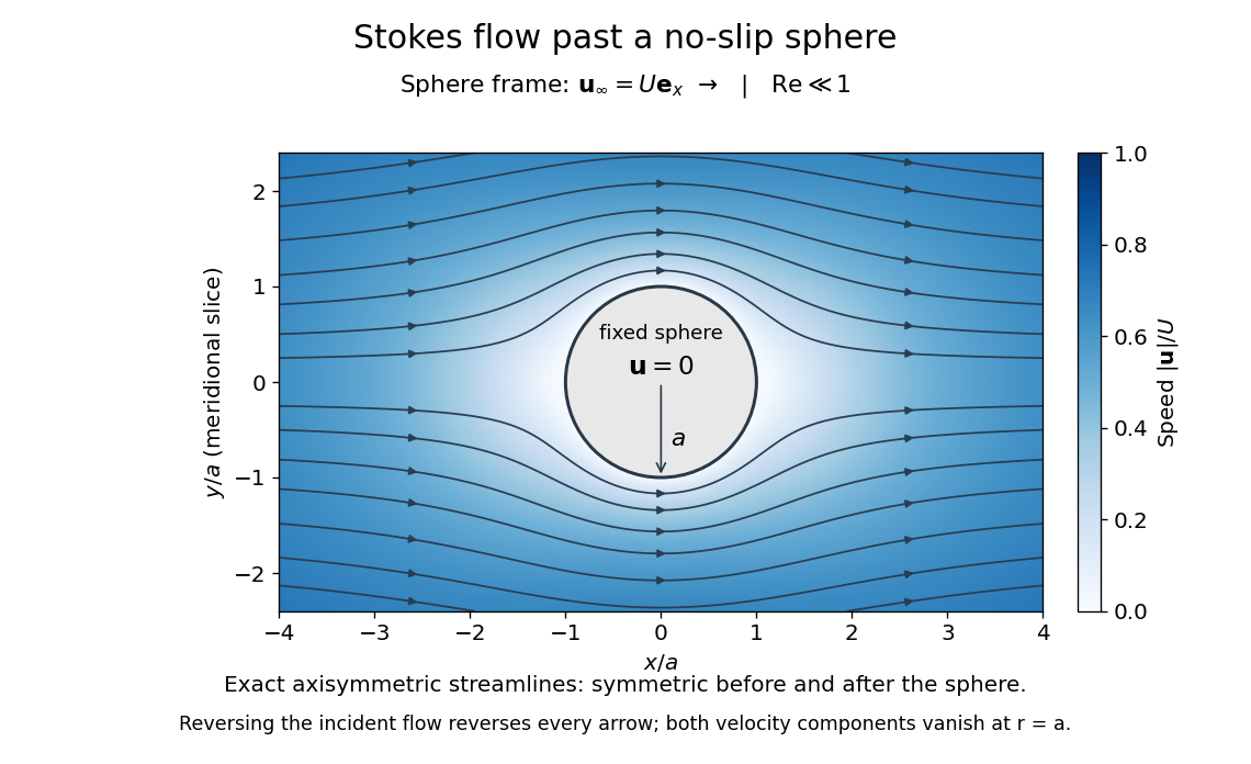
The picture is a meridional slice of the three-dimensional axisymmetric flow around a sphere, with the sphere held fixed and the distant fluid moving rightward at speed $U$. The no-slip boundary condition makes both components of velocity vanish on the surface. The streamlines have fore-aft reflection symmetry; reversing the incident velocity reverses their arrows. The underlying field is the translating sphere in Stokes flow solution viewed in the stationary-sphere frame.

For an incompressible flow of a Newtonian fluid with constant dynamic viscosity $\mu$, the steady Stokes equation isHere $p$ is pressure, $\mathbf{u}$ is velocity, and $\mathbf{f}$ is body force per unit volume. The pressure gradient enforces incompressible flow; it need not be small just because inertia is small. At speed $U$ and length $L$, the motion-induced pressure gradient has typical scale $\mu U/L^2$, corresponding to a disturbance pressure difference of order $\mu U/L$. See Shreyas Mandre's fluid dynamics notes, sections 9.1.1–9.1.2.

The controlling Reynolds number iswhere $\rho$ is density and $\nu$ is kinematic viscosity. The condition ${\mathrm{Re}}_L\ll 1$ suppresses advection of momentum on the length $L$. Rapid changes require an additional check of the viscous diffusion time: small Reynolds number alone does not eliminate the time derivative in the Unsteady Stokes equation.

Two rewards of this limit are the exact Stokes's law for the drag on a sphere and kinematic reversibility of Stokes flow. The first predicts settling velocities and connects to the Stokes–Einstein relation; the second explains why a microswimmer needs a nonreciprocal stroke, as expressed by the scallop theorem. Despite viscous dissipation, reversing the driving can retrace the motion: an especially striking consequence of Linearity of Stokes flow.

George Gabriel Stokes obtained the sphere drag and its terminal velocity in his 1851 investigation of how viscosity changes physical pendulum motion. He also used the slow fall of small water droplets to discuss clouds. The paper was read on 9 December 1850; 1851 is its publication date. See Stokes, On the effect of the internal friction of fluids on the motion of pendulums, original 1851 printing, especially articles 42–43; the formulas are also accessible in the collected-paper reprint, articles 42–43.

Module HT-03 covers fluid mechanics, hydraulic losses and centrifugal pumps. Printed pp.51–53 explain the system characteristic curve and pump operating point. The date in the current hosting path does not change the handbook's original publication year.

Weather forecasting estimates future meteorological conditions from observations and physical models. Numerical models use an approximate initial condition and equations of fluid mechanics to simulate future conditions; forecasters also compare model outputs and apply experience and research.^[ref] The forecast horizon describes how far ahead a prediction remains useful at a specified accuracy; sensitive dependence on initial conditions can limit detailed predictions under deterministic evolution.